
Statistics for Engineers and Scientists
4th Edition
ISBN: 9780073401331
Author: William Navidi Prof.
Publisher: McGraw-Hill Education
expand_more
expand_more
format_list_bulleted
Concept explainers
Videos
Textbook Question
Chapter 7.4, Problem 1E
The following output (from MINITAB) is for the least-squares fit of the model ln y = β0 + β1 ln x + ε, where y represents the monthly production of a gas well and x represents the volume of fracture fluid pumped in. (A
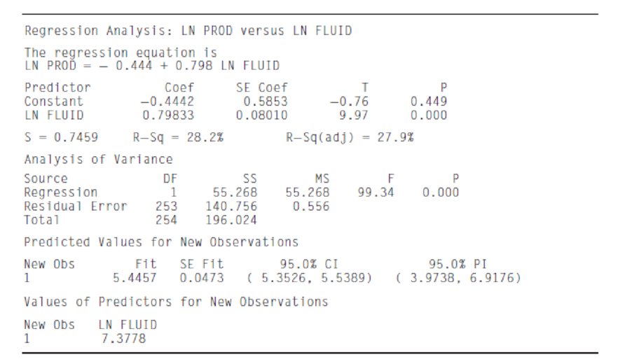
- a. What is the equation of the least-squares line for predicting ln y from ln x?
- b. Predict the production of a well into which 2500 gal/ft of fluid have been pumped.
- c. Predict the production of a well into which 1600 gal/ft of fluid have been pumped.
- d. Find a 95% prediction interval for the production of a well into which 1600 gal/ft of fluid have been pumped. (Note: In 1600 = 7.3778.)
Expert Solution & Answer
Want to see the full answer?
Check out a sample textbook solution
Students have asked these similar questions
Question 1
Provide an algebraic proof that the least squares estimator is not consistent when Cov(x,e)=0 with the regression model y =B1+B2E(x)+e where E(e)=0So that E(y) = B1 + B2E(x)
The following Minitab display gives information regarding the relationship between the body weight of a child (in kilograms) and the metabolic rate of the child (in 100 kcal/ 24 hr).
Predictor Coef SE Coef T PConstant 0.8570 0.4148 2.06 0.84Weight 0.38243 0.02978 13.52 0.000
S = 0.517508 R-Sq = 97.4%
(a) Write out the least-squares equation.
y^= ______ + _____x
(b) For each 1 kilogram increase in weight, how much does the metabolic rate of a child increase? (Use 5 decimal places.)
Table 14.17
The Least Squares Point Estimates for Exercise 14.51
Bo = 10.3676 (.3710)
B1 = .0500 (<.001)
B2 = 6.3218 (.0152)
B3 = -11.1032 (.0635)
B4 = -.4319 (.0002)
Questions
Using the t statistic and appropriate critical values, test Ho: βj = 0 versus Ha: βj ≠ 0 by setting α equal to .05. Which independent variables are significantly related to y in the model with α = .05?
Using the t statistic and appropriate critical values, test Ho: βj = 0 versus Ha: βj ≠ 0 by setting α equal to .01. Which independent variables are significantly related to y in the model with α = .01?
Find the p-value for testing Ho: βj = 0 versus Ha: βj ≠ 0 on the output. Using the p-value, determine whether we can reject Ho by setting α equal to .10, .05, .01, and .001. What do you conclude about the significance of the independent variables in the model?
Calculate the 95 percent confidence interval for βj. Discuss one practical application of this interval.
Calculate the 99 percent confidence interval for…
Chapter 7 Solutions
Statistics for Engineers and Scientists
Ch. 7.1 - Compute the correlation coefficient for the...Ch. 7.1 - For each of the following data sets, explain why...Ch. 7.1 - For each of the following scatterplots, state...Ch. 7.1 - True or false, and explain briefly: a. If the...Ch. 7.1 - In a study of ground motion caused by earthquakes,...Ch. 7.1 - A chemical engineer is studying the effect of...Ch. 7.1 - Another chemical engineer is studying the same...Ch. 7.1 - Tire pressure (in kPa) was measured for the right...Ch. 7.1 - Prob. 10ECh. 7.1 - The article Drift in Posturography Systems...
Ch. 7.1 - Prob. 12ECh. 7.1 - Prob. 13ECh. 7.1 - A scatterplot contains four points: (2, 2), (1,...Ch. 7.2 - Each month for several months, the average...Ch. 7.2 - In a study of the relationship between the Brinell...Ch. 7.2 - A least-squares line is fit to a set of points. If...Ch. 7.2 - Prob. 4ECh. 7.2 - In Galtons height data (Figure 7.1, in Section...Ch. 7.2 - In a study relating the degree of warping, in mm....Ch. 7.2 - Moisture content in percent by volume (x) and...Ch. 7.2 - The following table presents shear strengths (in...Ch. 7.2 - Structural engineers use wireless sensor networks...Ch. 7.2 - The article Effect of Environmental Factors on...Ch. 7.2 - An agricultural scientist planted alfalfa on...Ch. 7.2 - Curing times in days (x) and compressive strengths...Ch. 7.2 - Prob. 13ECh. 7.2 - An engineer wants to predict the value for y when...Ch. 7.2 - A simple random sample of 100 men aged 2534...Ch. 7.2 - Prob. 16ECh. 7.3 - A chemical reaction is run 12 times, and the...Ch. 7.3 - Structural engineers use wireless sensor networks...Ch. 7.3 - Prob. 3ECh. 7.3 - Prob. 4ECh. 7.3 - Prob. 5ECh. 7.3 - Prob. 6ECh. 7.3 - The coefficient of absorption (COA) for a clay...Ch. 7.3 - Prob. 8ECh. 7.3 - Prob. 9ECh. 7.3 - Three engineers are independently estimating the...Ch. 7.3 - In the skin permeability example (Example 7.17)...Ch. 7.3 - Prob. 12ECh. 7.3 - In a study of copper bars, the relationship...Ch. 7.3 - Prob. 14ECh. 7.3 - In the following MINITAB output, some of the...Ch. 7.3 - Prob. 16ECh. 7.3 - In order to increase the production of gas wells,...Ch. 7.4 - The following output (from MINITAB) is for the...Ch. 7.4 - The processing of raw coal involves washing, in...Ch. 7.4 - To determine the effect of temperature on the...Ch. 7.4 - The depth of wetting of a soil is the depth to...Ch. 7.4 - Good forecasting and control of preconstruction...Ch. 7.4 - The article Drift in Posturography Systems...Ch. 7.4 - Prob. 7ECh. 7.4 - Prob. 8ECh. 7.4 - A windmill is used to generate direct current....Ch. 7.4 - Two radon detectors were placed in different...Ch. 7.4 - Prob. 11ECh. 7.4 - The article The Selection of Yeast Strains for the...Ch. 7.4 - Prob. 13ECh. 7.4 - The article Characteristics and Trends of River...Ch. 7.4 - Prob. 15ECh. 7.4 - The article Mechanistic-Empirical Design of...Ch. 7.4 - An engineer wants to determine the spring constant...Ch. 7 - The BeerLambert law relates the absorbance A of a...Ch. 7 - Prob. 2SECh. 7 - Prob. 3SECh. 7 - Refer to Exercise 3. a. Plot the residuals versus...Ch. 7 - Prob. 5SECh. 7 - The article Experimental Measurement of Radiative...Ch. 7 - Prob. 7SECh. 7 - Prob. 8SECh. 7 - Prob. 9SECh. 7 - Prob. 10SECh. 7 - The article Estimating Population Abundance in...Ch. 7 - A materials scientist is experimenting with a new...Ch. 7 - Monitoring the yield of a particular chemical...Ch. 7 - Prob. 14SECh. 7 - Refer to Exercise 14. Someone wants to compute a...Ch. 7 - Prob. 16SECh. 7 - Prob. 17SECh. 7 - Prob. 18SECh. 7 - Prob. 19SECh. 7 - Use Equation (7.34) (page 545) to show that 1=1.Ch. 7 - Use Equation (7.35) (page 545) to show that 0=0.Ch. 7 - Prob. 22SECh. 7 - Use Equation (7.35) (page 545) to derive the...
Additional Math Textbook Solutions
Find more solutions based on key concepts
Use the model developed in Example 1.5 to predict the total sales for weeks 2 through 16, and compare the resul...
Business Analytics
Teacher Salaries
The following data from several years ago represent salaries (in dollars) from a school distri...
Elementary Statistics: A Step By Step Approach
Teacher Salaries
The following data from several years ago represent salaries (in dollars) from a school distri...
Elementary Statistics: A Step By Step Approach
Refer to the Real Estate data, which reports information on homes sold in the Goodyear, Arizona, area during th...
Statistical Techniques in Business and Economics
Medication Usage In a survey of 3005 adults aged 57 through 85 years, it was found that 82% of them used at lea...
Statistical Reasoning for Everyday Life (5th Edition)
TRY IT YOURSELF 2
Determine whether each number describes a population parameter or a sample statistic. Explain...
Elementary Statistics: Picturing the World (7th Edition)
Knowledge Booster


Learn more about
Need a deep-dive on the concept behind this application? Look no further. Learn more about this topic, statistics and related others by exploring similar questions and additional content below.Similar questions
- Consider the following table containing unemployment rates for a 10-year period. Unemployment Rates Year Unemployment Rate (%) 1 5.85.8 2 3.23.2 3 5.55.5 4 8.68.6 5 6.16.1 6 6.86.8 7 7.57.5 8 5.25.2 9 11.111.1 10 7.47.4 Step 1 of 2 : Given the model Estimated Unemployment Rate=β0+β1(Year)+εi,Estimated Unemployment Rate=�0+�1(Year)+��, write the estimated regression equation using the least squares estimates for β0�0 and β1�1. Round your answers to two decimal places.arrow_forwardConsider the following regression model Yt = β0 + β1 Ut + β2 Vt + β3 Wt + β4Xt + ∈t , where U, V, W, X and Y are economic variables observed from t = 1, . . . , 75, β0 , . . . , β4 are the model parameters and ∈t is the random disturbance term satisfying the classical assumptions. Ordinary Least Squares (OLS) is used to estimate the parameters, producing the following estimated model: Yt = 1.115 + 0.790*Ut − 0.327*Vt + 0.763*Wt + 0.456*Xt (0.405) (0.178) (0.088) (0.274) (0.017) where standard errors are given in parentheses, the R-squared = 0.941, the Durbin-Watson statistic is DW = 1.907 and the residual sum of squares is RSS = 0.0757. In answering this question, use the 5% level of significance for any hypothesis tests that you are asked to perform, state clearly the null and al- ternative hypotheses that you are testing, the test statistics that you are using and interpret the decisions that you make.…arrow_forwardThe following Minitab display gives information regarding the relationship between the body weight of a child (in kilograms) and the metabolic rate of the child (in 100 kcal/ 24 hr). Predictor Coef SE Coef T P Constant 0.8489 0.4148 2.06 0.84 Weight 0.39782 0.02978 13.52 0.000 S = 0.517508 R-Sq = 96.6% (a) Write out the least-squares equation. = + x (b) For each 1 kilogram increase in weight, how much does the metabolic rate of a child increase? (Use 5 decimal places.)(c) What is the value of the correlation coefficient r? (Use 3 decimal places.)arrow_forward
- In Galton’s height data (Figure 7.1, in Section 7.1), the least-squares line for predictingforearm length (y) from height (x) is y = −0.2967 + 0.2738x.a) Predict the forearm length of a man whose height is 70 in.b) How tall must a man be so that we would predict his forearm length to be 19 in.?c) All the men in a certain group have heights greater than the height computed in part(b). Can you conclude that all their forearms will be at least 19 in. long? Explain.arrow_forwardThe following table lists the birth weights (in pounds), x, and the lengths (in inches), y, for a set of newborn babies at a local hospital. Birth Weights and Lengths Birth Weight (in Pounds), x 6 11 5 3 9 12 11 11 4 10 Length (in Inches), y 16 18 15 15 20 20 19 20 16 21 Step 1 of 2 : Find an equation of the least-squares regression line. Round your answer to three decimal places, if necessary.arrow_forwardFor the following data set: x 3.9 6.1 4.6 3.7 1.8 3.3 3.4 y 4.2 4.7 5.7 4.5 9.6 5.2 4.3 Part 1 of 4 (a) Compute the least-squares regression line. Round the answers to at least four decimal places. Regression line equation: =y .arrow_forward
- Consider the following two a.m. peak work trip generation models, estimated by household linear regression: T = 0.62 + 3.1 X1 + 1.4 X2 R2= 0.590 (2.3) (7.1) (5.9) T = 0.01 + 2.4 X1 + 1.2 Z1 + 4.0 Z2 R2= 0.598 (0.8) (4.2) (1.7) (3.1) X1 = number of workers in the household X2 = number of cars in the household, Z1 is a dummy variable which takes the value 1 if the household has one car, Z2 is a dummy variable which takes the value 1 if the household has two or more cars. Compare the two models and choose the best. If a zone has 1000 households, of which 50% have no car, 35% have one car, and the rest have exactly two cars, estimate the total number of trips generated by this zone. Use the preferred trip generation model and assume that each household has an average of two workersarrow_forwardThe following table lists the birth weights (in pounds), x, and the lengths (in inches), y, for a set of newborn babies at a local hospital. Birth Weights and Lengths Birth Weight (in Pounds), x 4 8 10 4 12 7 10 10 6 5 Length (in Inches), y 16 20 18 17 21 19 19 20 18 15 Step 1 of 2 : Find an equation of the least-squares regression line. Round your answer to three decimal places, if necessary. instructions for if/how to do this on the TI84 would be greatly appreciated :)arrow_forwardFind the least-squares equation for the following pairs of data: x = earthquake magnitude 2.9 4.2 3.3 4.5 2.6 3.2 3.4 y = depth of earthquake (in km) 5 10 11.2 10 7.9 3.9 5.5 A. y = 2.16 + 0.221x B. y = 0.221 + 2.16x C. y = 2.16 + 0.312x D. y = 0.221 + 2.82xarrow_forward
- If a set of paired data gives the indication that the regression equation is of the form μY|x = α · βx, it is cus-tomary to estimate α and β by fitting the line log ˆy = log ˆα + x · log βˆ to the points {(xi, log yi);i = 1, 2, ... , n} by the methodof least squares. Use this technique to fit an exponentialcurve of the form ˆy = αˆ · βˆx to the following data on thegrowth of cactus grafts under controlled environmentalconditions: Weeks after Heightgrafting (inches)x y1 2.02 2.44 5.15 7.36 9.48 18.3arrow_forwardFor some genetic mutations, it is thought that the frequency of the mutant gene in men increases linearly with age. If m1 is the frequency at age t1, and m2 is the frequency at age t2, then the yearly rate of increase is estimated by r = (m2 − m1)/(t2 − t1). In a polymerase chain reaction assay, the frequency in 20-year-old men was estimated to be 17.7 ± 1.7 per μgDNA, and the frequency in 40-year-old men was estimated to be 35.9 ± 5.8 per μg DNA. Assume that age is measured with negligible uncertainty.a) Estimate the yearly rate of increase, and find the uncertainty in the estimate.b) Find the relative uncertainty in the estimated rate of increase.arrow_forwardA Sociologist wishes to see whether the number of years of schooling a person has is dependent on the person’s location. The information is classified as follows: Location No education Four-year degree Advanced degree Total Metropolis 15 12 8 35 Suburban 8 15 9 32 Countryside 6 8 7 21 Total 29 35 24 88 At alpha 0.05, can the Sociologist conclude that a person’s location is dependent on the number of years of schooling? Find p-value and on the basis of the p-value, should the null hypothesis be rejected?arrow_forward
arrow_back_ios
SEE MORE QUESTIONS
arrow_forward_ios
Recommended textbooks for you
 Linear Algebra: A Modern IntroductionAlgebraISBN:9781285463247Author:David PoolePublisher:Cengage Learning
Linear Algebra: A Modern Introduction
Algebra
ISBN:9781285463247
Author:David Poole
Publisher:Cengage Learning
Correlation Vs Regression: Difference Between them with definition & Comparison Chart; Author: Key Differences;https://www.youtube.com/watch?v=Ou2QGSJVd0U;License: Standard YouTube License, CC-BY
Correlation and Regression: Concepts with Illustrative examples; Author: LEARN & APPLY : Lean and Six Sigma;https://www.youtube.com/watch?v=xTpHD5WLuoA;License: Standard YouTube License, CC-BY