Statistics for Engineers and Scientists (Looseleaf)
4th Edition
ISBN: 9780073515687
Author: Navidi
Publisher: MCG
expand_more
expand_more
format_list_bulleted
Videos
Textbook Question
Chapter 7.4, Problem 14E
The article “Characteristics and Trends of River Discharge into Hudson, James, and Ungava Bays, 1964–2000” (S. Déry, M. Stieglitz, et al., Journal of Climate, 2005:2540–2557) presents measurements of discharge rate x (in km3/yr) and peak flow y (in m3/s) for 42 rivers that drain into the Hudson, James, and Ungava Bays. The data are shown in the following table:
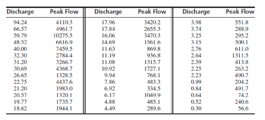
- a. Compute the least-squares line for predicting y from x. Make a plot of residuals versus fitted values.
- b. Compute the least-squares line for predicting y from ln x. Make a plot of residuals versus fitted values.
- c. Compute the least-squares line for predicting ln y from ln x. Make a plot of residuals versus fitted values.
- d. Which of the three models (a) through (c) fits best? Explain.
- e. Using the best model, predict the peak flow when the discharge is 50.0 km3/yr.
- f. Using the best model, find a 95% prediction interval for the peak flow when the discharge is 50.0 km3/yr.
Expert Solution & Answer
Want to see the full answer?
Check out a sample textbook solution
Students have asked these similar questions
The article "Characteristics and Trends of River Discharge into Hudson, James, and Ungava
Bays, 1964-2000" (S. Dery, M. Stieglitz, et al., Journal of Climate, 2005:2540-2557)
presents measurements of discharge rate x (in kmlyr) andpeakflow y (in m/s) for 42 rivers
that drain into the Hudson, James, and Ungava Bays. The data are shown in the following
table:
Discharge
Peak Flow
94.24
4110.3
66.57
4961.7
59.79
10275.5
48.52
6616.9
40.00
7459.5
32.30
2784.4
31.20
3266.7
30.69
4368.7
26.65
1328.5
22.75
4437.6
21.20
1983.0
20.57
1320.1
19.77
1735.7
18.62
1944.1
17.96
3420.2
17.84
2655.3
16.06
3470.3
1561.6
14.69
11.63
869.8
11.19
936.8
11.08
1315.7
10.92
1727.1
9.94
768.1
7.86
483.3
An article in the Journal of Environmental Engineering (1989, Vol. 115(3), pp.
608–619) reported the results of a study on the occurrence of sodium and chloride in surface
streams in central Rhode Island. The following data are chloride concentration y (in milligrams per
liter) and roadway area in the watershed x (in percentage).
An article in Air and Waste ("Update on Ozone Trends in California's South Coast Air Basin," Vol. 43, 1993) studied the ozone levels
on the South Coast air basin of California for the years 1976-1991. The author believes that the number of days that the ozone
exceeds 0.20 parts per million depends on the seasonal meteorological index (the seasonal average 850 millibar temperature). The
data follow:
Year Days Index
16.3
1976 91
1977 105 17.1
1978 106 18.2
1979 108 18.1
1980 88
17.2
1981 91
18.2
1982 58
16.0
1983 82 17.2
Round your answers to 2 decimal places.
(a) Fit a simple linear regression model to the data. Test for significance of regression using a = 0.05.
y = i
Calculate fo: i
Year Days Index
1984 82
17.7
1985 65
17.2
1986 61
16.9
1987
48
17.1
1988 61
18.2
1989 43 17.3
1990 33 17.5
1991 36
16.6
i
+ i
Is the simple linear regression model significant? No.
(b) Calculate a 95% confidence interval on the slope.
≤B₁ ≤i
X
Chapter 7 Solutions
Statistics for Engineers and Scientists (Looseleaf)
Ch. 7.1 - Compute the correlation coefficient for the...Ch. 7.1 - For each of the following data sets, explain why...Ch. 7.1 - For each of the following scatterplots, state...Ch. 7.1 - True or false, and explain briefly: a. If the...Ch. 7.1 - In a study of ground motion caused by earthquakes,...Ch. 7.1 - A chemical engineer is studying the effect of...Ch. 7.1 - Another chemical engineer is studying the same...Ch. 7.1 - Tire pressure (in kPa) was measured for the right...Ch. 7.1 - Prob. 10ECh. 7.1 - The article Drift in Posturography Systems...
Ch. 7.1 - Prob. 12ECh. 7.1 - Prob. 13ECh. 7.1 - A scatterplot contains four points: (2, 2), (1,...Ch. 7.2 - Each month for several months, the average...Ch. 7.2 - In a study of the relationship between the Brinell...Ch. 7.2 - A least-squares line is fit to a set of points. If...Ch. 7.2 - Prob. 4ECh. 7.2 - In Galtons height data (Figure 7.1, in Section...Ch. 7.2 - In a study relating the degree of warping, in mm....Ch. 7.2 - Moisture content in percent by volume (x) and...Ch. 7.2 - The following table presents shear strengths (in...Ch. 7.2 - Structural engineers use wireless sensor networks...Ch. 7.2 - The article Effect of Environmental Factors on...Ch. 7.2 - An agricultural scientist planted alfalfa on...Ch. 7.2 - Curing times in days (x) and compressive strengths...Ch. 7.2 - Prob. 13ECh. 7.2 - An engineer wants to predict the value for y when...Ch. 7.2 - A simple random sample of 100 men aged 2534...Ch. 7.2 - Prob. 16ECh. 7.3 - A chemical reaction is run 12 times, and the...Ch. 7.3 - Structural engineers use wireless sensor networks...Ch. 7.3 - Prob. 3ECh. 7.3 - Prob. 4ECh. 7.3 - Prob. 5ECh. 7.3 - Prob. 6ECh. 7.3 - The coefficient of absorption (COA) for a clay...Ch. 7.3 - Prob. 8ECh. 7.3 - Prob. 9ECh. 7.3 - Three engineers are independently estimating the...Ch. 7.3 - In the skin permeability example (Example 7.17)...Ch. 7.3 - Prob. 12ECh. 7.3 - In a study of copper bars, the relationship...Ch. 7.3 - Prob. 14ECh. 7.3 - In the following MINITAB output, some of the...Ch. 7.3 - Prob. 16ECh. 7.3 - In order to increase the production of gas wells,...Ch. 7.4 - The following output (from MINITAB) is for the...Ch. 7.4 - The processing of raw coal involves washing, in...Ch. 7.4 - To determine the effect of temperature on the...Ch. 7.4 - The depth of wetting of a soil is the depth to...Ch. 7.4 - Good forecasting and control of preconstruction...Ch. 7.4 - The article Drift in Posturography Systems...Ch. 7.4 - Prob. 7ECh. 7.4 - Prob. 8ECh. 7.4 - A windmill is used to generate direct current....Ch. 7.4 - Two radon detectors were placed in different...Ch. 7.4 - Prob. 11ECh. 7.4 - The article The Selection of Yeast Strains for the...Ch. 7.4 - Prob. 13ECh. 7.4 - The article Characteristics and Trends of River...Ch. 7.4 - Prob. 15ECh. 7.4 - The article Mechanistic-Empirical Design of...Ch. 7.4 - An engineer wants to determine the spring constant...Ch. 7 - The BeerLambert law relates the absorbance A of a...Ch. 7 - Prob. 2SECh. 7 - Prob. 3SECh. 7 - Refer to Exercise 3. a. Plot the residuals versus...Ch. 7 - Prob. 5SECh. 7 - The article Experimental Measurement of Radiative...Ch. 7 - Prob. 7SECh. 7 - Prob. 8SECh. 7 - Prob. 9SECh. 7 - Prob. 10SECh. 7 - The article Estimating Population Abundance in...Ch. 7 - A materials scientist is experimenting with a new...Ch. 7 - Monitoring the yield of a particular chemical...Ch. 7 - Prob. 14SECh. 7 - Refer to Exercise 14. Someone wants to compute a...Ch. 7 - Prob. 16SECh. 7 - Prob. 17SECh. 7 - Prob. 18SECh. 7 - Prob. 19SECh. 7 - Use Equation (7.34) (page 545) to show that 1=1.Ch. 7 - Use Equation (7.35) (page 545) to show that 0=0.Ch. 7 - Prob. 22SECh. 7 - Use Equation (7.35) (page 545) to derive the...
Additional Math Textbook Solutions
Find more solutions based on key concepts
z Scores. In Exercises 5-8, express all z scores with two decimal places.
8. Plastic Waste Data Set 31 “Garbage...
Elementary Statistics Using Excel (6th Edition)
How much time do Americans living in or near cities spend waiting in traffic, and how much does waiting in traf...
Business Statistics: A First Course (7th Edition)
The data in Table 1A were collected from one of the authors’ statistics classes. The first row gives the variab...
Introductory Statistics
Use the model developed in Example 1.5 to predict the total sales for weeks 2 through 16, and compare the resul...
Business Analytics
Testing Hypotheses. In Exercises 13-24, assume that a simple random sample has been selected and test the given...
Elementary Statistics Using the TI-83/84 Plus Calculator, Books a la Carte Edition (4th Edition)
Knowledge Booster


Learn more about
Need a deep-dive on the concept behind this application? Look no further. Learn more about this topic, statistics and related others by exploring similar questions and additional content below.Similar questions
- An article in the ASCE Journal of Energy Engineering [“Overview of Reservoir Release Improvements at 20 TVA Dams” (Vol. 125, April 1999, pp. 1–17)] presents data on dissolved oxygen concentrations in streams below 20 dams in the Tennessee Valley Authority system. The observations are (in milligrams per liter):arrow_forwardThe article “‘Little Ice Age’ Proxy Glacier Mall Balance Records Reconstructed from Tree Rings in the Mt. Waddington Area, British Columbia Coast Mountains, Canada” (S. Larocque and D. Smith, The Holocene, 2005:748–757) evaluates the use of tree ring widths to estimate changes in the masses of glaciers. For the Sentinel glacier, the net mass balance (change in mass between the end of one summer and the end of the next summer) was measured for 23 years. During the same time period, the tree ring index for white bark pine trees was measured, and the sample correlation between net mass balance and tree ring index was r = −0.509. Can you conclude that the population correlation ρ differs from 0?arrow_forwardA sociologist wants to determine if the life expectancy of people in Africa is less than the life expectancy of people in Asia. The data obtained is shown in the table below. Africa Asia = 63.3 yr. 1 X,=65.2 yr. 2 o, = 9.1 yr. = 7.3 yr. n1 = 120 = 150arrow_forward
- Following are measurements of soil concentrations (in mg /kg) of chromium (Cr) and nickel (Ni) at20 sites in the area of Cleveland, Ohio. These data are taken from the article "Variation in NorthAmerican Regulatory Guidance for Heavy Metal Surface Soil Contamination at Commercial andIndustrial Sites" (A. Jennings and J. Ma, J. Environment Eng, 2007:587-609). Cr: 260 19 36 247 263 319 317 277 319 264 23 29 61 119 33 281 21 35 64 30Ni: 435 377 359 53 38 38 54 188 397 33 92 490 28 35 799 347 321 32 74 508 (a) Construct a histogram for each set of concentrations. (b) Find the 1st, 2nd and 3rd quartiles for the Cr concentrations (c) Find the 1st, 2nd and 3rd quartiles for the Ni concentrations.arrow_forwardA study was performed looking at the risk of fractures in three rural Iowa communities according to whether their drinking water was “higher calcium,” “higher fluorides,” or “control” as determined by water samples. Table 11.10 presents data comparing the rate of fractures (over 5 years) between the higher-calcium vs the control communities for women ages 20–35 and 55–80, respectively . Table 11.10 Relationship of calcium content of drinking water to the rate of fractures in rural Iowa Ages 20-35 Number of women with fractures Total number of women Ages 55-80 Number of woemn with fractures Total number of women Control 3 37 Control 11 121 High calcium 1 33 High calcium 21 148 13.1 What test can be used to compare the fracturerates in these two communities while controlling for age? 13.2 Implement the test in Problem 13.1, report a p-value, and make a conclusion on relationship between drinking water calcium concentration and rate of fracture based on the p-value.arrow_forwardFollowing are measurements of soil concentrations (in mg /kg) of chromium (Cr) and nickel (Ni) at20 sites in the area of Cleveland, Ohio. These data are taken from the article "Variation in NorthAmerican Regulatory Guidance for Heavy Metal Surface Soil Contamination at Commercial andIndustrial Sites" (A. Jennings and J. Ma, J. Environment Eng, 2007:587-609).Cr: 260 19 36 247 263 319 317 277 319 264 23 29 61 119 33 281 21 35 64 30Ni: 435 377 359 53 38 38 54 188 397 33 92 490 28 35 799 347 321 32 74 508 (d) Use these to construct comparative boxplots for the two sets of concentrations. (e) Using the boxplots, what differences can be seen between the two sets of concentrations?arrow_forward
- A study was performed looking at the risk of fractures in three rural Iowa communities according to whether their drinking water was “higher calcium,” “higher fluorides,” or “control” as determined by water samples. Table 11.10 presents data comparing the rate of fractures (over 5 years) between the higher-calcium vs the control communities for women ages 20–35 and 55–80, respectively . Table 11.10 Relationship of calcium content of drinking water to the rate of fractures in rural Iowa Ages 20-35 Number of women with fractures Total number of women Ages 55-80 Number of woemn with fractures Total number of women Control 3 37 Control 11 121 High calcium 1 33 High calcium 21 148 13.1 What test can be used to compare the fracturerates in these two communities while controlling for age? 13.2 Implement the test in Problem 13.1, report a p-value, and make a conclusion on relationship between drinking water calcium concentration and rate of fracture based on the p-value. 13.3…arrow_forwardCell Phone Radiation Listed below are the measured radiation absorption rates (in W/kg) corresponding to these cell phones: iPhone 5S, BlackBerry Z30, Sanyo Vero, Optimus V, Droid Razr, Nokia N97, Samsung Vibrant, Sony Z750a, Kyocera Kona, LG G2, and Virgin Mobile Supreme. The data are from the Federal Communications Commission (FCC). The media often report about the dangers of cell phone radiation as a cause of cancer. The FCC has a standard that a cell phone absorption rate must be 1.6 W/kg or less. If you are planning to purchase a cell phone, are any of the measures of center the most important statistic? Is there another statistic that is most relevant? If so, which one?arrow_forwardAn article in the journal Air and Waste (Update on Ozone Trends in California's South Coast Air Basin, Vol. 43, 1993) investigated the ozone levels in the South Coast Air Basin of California for the years 1976-1991. The author believes that the number of days the ozone levels exceeded 0.20 ppm (the response) depends on the seasonal meteorological index, which is the seasonal average 850-millibar Temperature (the predictor). The following table gives the data. Year Index 1976 1977 1978 1979 1980 1981 1982 1983 1984 1985 1986 1987 1988 1989 1990 1991 Days 91 105 106 108 88 91 58 82 81 65 61 48 61 43 33 36 16.7 17.1 18.2 18.1 17.2 18.2 16.0 17.2 18.0 17.2 16.9 17.1 18.2 17.3 17.5 16.6 (a) Construct a scatter diagram of the data. (b) Estimate the prediction equation. (c) Test for significance of regression. (d) Calculate the 95% CI and PI on for a seasonal meteorological index value of 17. Interpret these quantities.arrow_forward
- Alcohol use in the United States increased during the first year of the COVID pandemic, as did the number of alcohol-induced deaths (such as alcoholic liver disease, accidental alcohol poisoning, disorders due to acute intoxication). Here is a figure from the CDC representing the "Rates of alcohol-induced deaths in the United States in 2020, broken down by sex and age group." Figure 2. Rates of alcohol-induced deaths, by sex and age group: United States, 2020 Age group (years) Under 25 0.1 25-34 35-44 45-54 55-64 65-74 75-84 85 and over Under 25 25-34 35-44 45-54 55-64 65-74 75-84 85 and over 0 0.3 3.9 2.9 6.4 10.2 7.9 10 12.9 12.8 16.7 20 21.0 21.8 24.5 Female Male 38.5 SOURCE: National Center for Health Statistics, National Vital Statistics System, Mortality. I 40 43.4 30 Deaths per 100,000 population 50 59.0 I 60 70 Interpret the bottom-most bar (gray bar with the value "12.8" written next to it) as a sentence in context. Enter your answer here Select ALL correct interpretations of…arrow_forwardThe article "Influence of Freezing Temperature on Hydraulic Conductivity of Silty Clay" (J. Konrad and M. Samson, Journal of Geotechnical and Geoenvironmental Engineering, 2000:180–187) describes a study of factors affecting hydraulic conductivity of soils. The measurements of hydraulic conductivity in units of 108 cm/s (y), initial void ratio (x), and thawed void ratio (x2) for 12 specimens of silty clay are presented in the following table. y 1.01 1.12 1.04 1.30 1.01 1.04 0.955 1.15 1.23 1.28 1.23 1.30 0.84 0.88 0.85 0.95 0.88 0.86 0.85 0.89 0.90 0.94 0.88 0.90 X1 0.81 0.85 0.87 0.92 0.84 0.85 0.85 0.86 0.85 0.92 0.88 0.92 X2 Fit the model y = Bo + fix1 + e. For each coefficient, test the null hypothesis that it is equal to 0. Fit the model y = Bo + Bzx2 + e. For each coefficient, test the null hypothesis that it is equal to 0. Fit the model y = Bo + BzX1 + Bzxz + e. For each coefficient, test the null hypothesis that it is equal to 0. d. Which of the models in parts (a) to (c) is…arrow_forwardAn article in the Fire Safety Journal (“The Effect of Nozzle Design on the Stability and Performance of Turbulent Water Jets,” Vol. 4, August 1981) describes an experiment in which a shape factor was determined for several different nozzle designs at six levels of jet efflux velocity. Interest focused on potential differences between nozzle designs (blocks), with velocity considered as a nuisance variable. The data are shown below: Jet Efflux Velocity (m/s) Nozzle Design 11.73 14.37 16.59 20.43 23.46 28.74 1 0.78 0.80 0.81 0.75 0.77 0.78 2 0.85 0.85 0.92 0.86 0.81 0.83 3 0.93 0.92 0.95 0.89 0.89 0.83 4 1.14 0.97 0.98 0.88 0.86 0.83 5 0.97 0.86 0.78 0.76 0.76 0.75 1) Write the null hypothesis and the alternative hypothesis (for the factor). 2) Find the ANOVA table. (round to five decimal places). 3) What is your decision about the null hypothesis, consider ?. 4) If your decision in part (4) was reject , perform Tukey test to determine which pairwise means are…arrow_forward
arrow_back_ios
SEE MORE QUESTIONS
arrow_forward_ios
Recommended textbooks for you
 MATLAB: An Introduction with ApplicationsStatisticsISBN:9781119256830Author:Amos GilatPublisher:John Wiley & Sons Inc
 Probability and Statistics for Engineering and th...StatisticsISBN:9781305251809Author:Jay L. DevorePublisher:Cengage Learning
 Statistics for The Behavioral Sciences (MindTap C...StatisticsISBN:9781305504912Author:Frederick J Gravetter, Larry B. WallnauPublisher:Cengage Learning
 Elementary Statistics: Picturing the World (7th E...StatisticsISBN:9780134683416Author:Ron Larson, Betsy FarberPublisher:PEARSON
 The Basic Practice of StatisticsStatisticsISBN:9781319042578Author:David S. Moore, William I. Notz, Michael A. FlignerPublisher:W. H. Freeman
 Introduction to the Practice of StatisticsStatisticsISBN:9781319013387Author:David S. Moore, George P. McCabe, Bruce A. CraigPublisher:W. H. Freeman
MATLAB: An Introduction with Applications
Statistics
ISBN:9781119256830
Author:Amos Gilat
Publisher:John Wiley & Sons Inc
Probability and Statistics for Engineering and th...
Statistics
ISBN:9781305251809
Author:Jay L. Devore
Publisher:Cengage Learning
Statistics for The Behavioral Sciences (MindTap C...
Statistics
ISBN:9781305504912
Author:Frederick J Gravetter, Larry B. Wallnau
Publisher:Cengage Learning
Elementary Statistics: Picturing the World (7th E...
Statistics
ISBN:9780134683416
Author:Ron Larson, Betsy Farber
Publisher:PEARSON
The Basic Practice of Statistics
Statistics
ISBN:9781319042578
Author:David S. Moore, William I. Notz, Michael A. Fligner
Publisher:W. H. Freeman
Introduction to the Practice of Statistics
Statistics
ISBN:9781319013387
Author:David S. Moore, George P. McCabe, Bruce A. Craig
Publisher:W. H. Freeman
Hypothesis Testing using Confidence Interval Approach; Author: BUM2413 Applied Statistics UMP;https://www.youtube.com/watch?v=Hq1l3e9pLyY;License: Standard YouTube License, CC-BY
Hypothesis Testing - Difference of Two Means - Student's -Distribution & Normal Distribution; Author: The Organic Chemistry Tutor;https://www.youtube.com/watch?v=UcZwyzwWU7o;License: Standard Youtube License