Concept explainers
Videos
Structural engineers use wireless sensor networks to monitor the condition of dams and bridges. The article “Statistical Analysis of Vibration
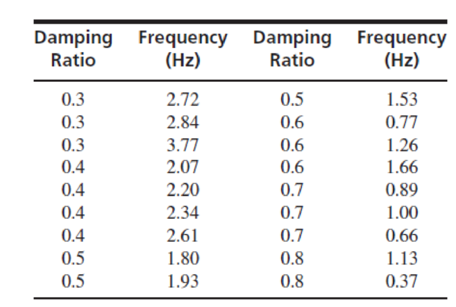
- a. Construct a
scatterplot of frequency (y) versus damping ratio (x). Verify that a linear model is appropriate. - b. Compute the least-squares line for predicting frequency from damping ratio.
- c. If two modes differ in damping ratio by 0.2, by how much would you predict their frequencies to differ?
- d. Predict the frequency for modes with damping ratio 0.75.
- e. Should the equation be used to predict the frequency for modes that are overdamped (damping ratio > 1)? Explain why or why not.
- f. For what damping ratio would you predict a frequency of 2.0?
Want to see the full answer?
Check out a sample textbook solution
Chapter 7 Solutions
Statistics for Engineers and Scientists (Looseleaf)
Additional Math Textbook Solutions
Statistical Reasoning for Everyday Life (5th Edition)
Fundamentals of Statistics (5th Edition)
Business Analytics
Research Methods for the Behavioral Sciences (MindTap Course List)
Elementary Statistics Using The Ti-83/84 Plus Calculator, Books A La Carte Edition (5th Edition)


- 5) Alcohol consumption is influenced by price and packaging, but what about glassware? Atwood et al. (2012) measured whether the time taken to drink a beer was influenced by the shape of the glass in which it was served. Participants were given a 12 oz. of chilled lager and were told that they should drink it at their own pace while watching a nature documentary. The participants were randomly assigned to receive their beer in either a straight-sided glass or a curved, fluted glass. The data below are the total time in minutes to drink the glass of beer by the 19 women participants in the study. Straight glass: 11.63 10.37 17.89 6.96 20.40 20.64 9.26 18.11 10.33 23.54 Curved glass: 7.46 9.28 8.90 6.73 8.25 6.16 13.09 2.10 6.37 a. Show the data in a graph. What trend is suggested? Comment on other differences between the frequency distributions of the two samples. b. Test whether the mean total time to drink the beer differs depending on beer glass shape.arrow_forwardBody Fat. In the paper “Total Body Composition by Dual- Photon (153 Gd) Absorptiometry” (American Journal of Clinical Nutrition, Vol. 40, pp. 834–839), R. Mazess et al. studied methods for quantifying body composition. Eighteen randomly selected adults were measured for percentage of body fat, using dual-photon absorptiometry. Each adult’s age and percentage of body fat are shown on the WeissStats site. a. Decide whether finding a regression line for the data is reasonable. If so, then also do parts (b)–(d). b. Obtain the coefficient of determination. c. Determine the percentage of variation in the observed values of the response variable explained by the regression, and interpret your answer. d. State how useful the regression equation appears to be for making predictions.arrow_forwardBody Fat. In the paper “Total Body Composition by Dual- Photon (153 Gd) Absorptiometry” (American Journal of Clinical Nutrition, Vol. 40, pp. 834–839), R. Mazess et al. studied methods for quantifying body composition. Eighteen randomly selected adults were measured for percentage of body fat, using dual-photon absorptiometry. Each adult’s age and percentage of body fat are shown on the WeissStats site. a. Decide whether you can reasonably apply the regression t-test. If so, then also do part (b). b. Decide, at the 5% significance level, whether the data provide sufficient evidence to conclude that the predictor variable is useful for predicting the response variable.arrow_forward
- The article “Approximate Methods for Estimating Hysteretic Energy Demand on PlanAsymmetric Buildings” (M. Rathhore, A. Chowdhury, and S. Ghosh, Journal of Earthquake Engineering, 2011: 99–123) presents a method, based on a modal pushover analysis, of estimating the hysteretic energy demand placed on a structure by an earthquake. A sample of 18 measurements had a mean error of 457.8 kNm with a standard deviation of 317.7 kNm. An engineer claims that the method is unbiased, in other words, that the mean error is 0. Can you conclude that this claim is false?arrow_forwardThe article "Combined Analysis of Real-Time Kinematic GPS Equipment and Its Users for Height Determination" (W. Featherstone and M. Stewart, Journal of Surveying Engineering, 2001:31-51) presents a study of the accuracy of global positioning system (GPS) equipment in measuring heights. Three types of equipment were studied, and each was used to make measurements at four different base stations (in the article a fifth station was included, for which the results differed considerably from the other four). There were 60 measurements made with each piece of equipment at each base. The means and standard deviations of the measurement errors (in mm) are presented in the following table for each combination of equipment type and base station. Instrument A Instrument B Instrument C Standard Mean Deviation Mean Deviation Mean Deviation 18 Standard Standard Base 3 15 -24 18 -6 Base 14 26 -13 13 -2 16 Base 26 -22 39 29 Base 34 -17 26 15 18 a Construct an ANOVA table. You may give ranges for the…arrow_forwardThe depth of wetting of a soil is the depth to which water content will increase owing to extemal factors. The article "Discussion of Method for Evaluation of Depth of Wetting in Residential Areas" (J. Nelson, K. Chao, and D. Overton, Journal of Geotechnical and Geoenvironmental Engineering, 2011:293-296) discusses the relationship between depth of wetting beneath a structure and the age of the structure. The article presents measurements of depth of wetting, in meters, and the ages, in years, of 21 houses, as shown in the following table. Age Depth 7.6 4 4.6 6.1 9.1 3 4.3 7.3 5.2 10.4 15.5 5.8 10.7 4 5.5 6.1 10.7 10.4 4.6 7.0 6.1 14 16.8 10 9.1 8.8 Compute the least-squares line for predicting depth of wetting (y) from age (x). b. Identify a point with an unusually large x-value. Compute the least-squares line that results from deletion of this point. Identify another point which can be classified as an outlier. Compute the least-squares line that results from deletion of the outlier,…arrow_forward
- NW 6.12 CORPORATE SUSTAINABILITY OF CPA FIRMS. Corporate sustainability refers to business practices designed CORSUS around social and environmental considerations. Refer to the Business and Society (March 2011) study on the sustainability behaviors of CPA corporations, Exercise 2.23 (p. 59). Recall that the level of support for corporate sustainability (measured on a quantitative scale ranging from 0 to 160 points) was obtained for each in a sample of 992 senior managers at CPA firms. Higher point values indicate a higher level of support for sustainability. The accompanying StatCrunch printout gives a 99% confidence interval for the mean level of support for all senior managers at CPA firms. One sample T confidence interval: μ: Mean of variable 99% confidence interval results: Variable Sample Mean Std. Err. DF L. Limit U. Limit Support 67.75504 0.85314633 991 65.553241 69.95684 a. Locate the 99% confidence interval on the printout. b. Use the sample mean and standard deviation on the…arrow_forwardThe degenerative disease osteoarthritis most frequently affects weight-bearing joints such as knee. The article “Evidence of Mechanical Load Redistribution at the Knee Joint in the Elderly when Ascending Stairs and Ramps” (Annals of Biomed. Engr., 2008:467-476) presented the following summary data on stance duration (ms) for samples of both older and younger adults. Age Sample Size Sample Mean Sample SD Older 28 801 117 Younger 16 780 72 Assume that both stance duration distributions are normal. Carry out a test of hypotheses at significance level .05 to decide whether true average stance duration is larger among elderly individuals than among younger individuals. (Population variances are not assumed equal.)arrow_forwardThe article "Application of Analysis of Variance to Wet Clutch Engagement" (M. Mansouri, M. Khonsari, et al., Proceedings of the Institution of Mechanical Engineers, 2002:117-125) presents the following fitted model for predicting clutch engagement time in seconds (y) from engagement starting speed in m/s (x1), maximum drive torque in N · m (x2), system inertia in kg · m² (x3), and applied force rate in kN/s (x4): y = -0.83 + 0.017.x, + 0.0895x, + 42.77.xz + 0.027x, – 0.0043x,x, The sum of squares for regression was SSR = 1.08613 and the sum of squares for error was SSE = 0.036310. There were 44 degrees of freedom for error. Predict the clutch engagement time when the starting speed is 20 m/s, the maximum drive torque is 17 N·m, the system inertia is 0.006 kg · m², and the applied force rate is 10 kN/s. b. Is it possible to predict the change in engagement time associated with an increase of 2 m/s in starting speed? If so, find the predicted change. If not, explain why not. Is it…arrow_forward
- Following are measurements of soil concentrations (in mg /kg) of chromium (Cr) and nickel (Ni) at20 sites in the area of Cleveland, Ohio. These data are taken from the article "Variation in NorthAmerican Regulatory Guidance for Heavy Metal Surface Soil Contamination at Commercial andIndustrial Sites" (A. Jennings and J. Ma, J. Environment Eng, 2007:587-609). Cr: 260 19 36 247 263 319 317 277 319 264 23 29 61 119 33 281 21 35 64 30Ni: 435 377 359 53 38 38 54 188 397 33 92 490 28 35 799 347 321 32 74 508 (a) Construct a histogram for each set of concentrations. (b) Find the 1st, 2nd and 3rd quartiles for the Cr concentrations (c) Find the 1st, 2nd and 3rd quartiles for the Ni concentrations.arrow_forwardAt what age do babies learn to crawl? Does it take longer to learn in the winter when babies are often bundled in clothes that restrict their movement? Data were collected from parents who brought their babies into the University of Denver Infant Study Center to participate in one of a number of experiments between 1988 and 1991. Parents reported the birth month and the age at which their child was first able to creep or crawl a distance of four feet within one minute. The resulting data were grouped by month of birth. The data are for January, May, and September AverageBirth month crawling age SD nJanuary 29.84 7.08 32May 28.58 8.07 27September 33.83 6.93 38 Crawling age is given in weeks. Assume the data come from three independent simple random samples, one from each of the three populations (babies born in a particular month) and that the populations of crawling ages have normal…arrow_forwardThe article "Effect of Environmental Factors on Steel Plate CoIrosion Under Marine Immersion Conditions" (C. Soares, Y. Garbatov, and A. Zayed, Corrosion Engineering, Science and Technology, 2011:524-541) descrībes an experiment in which nine steel specimens were submerged in seawater at various temperatures, and the corrosion rates were measured. The results are presented in the following table (obtained by digitizing a graph). Temperature (*C) Corrosion (mnm/yr) 26.6 1.58 26.0 1.45 27.4 1.13 21.7 0.96 14.9 0.99 11.3 1.05 15.0 0.82 8.7 0.68 8.2 0.56 Construct a scatterplot of corosion (y) versus temperature (x). Verify that a linear model is appropriate. Compute the least-squares line for predicting corrosion from temperature. Two steel specimens whose temperatures differ by 10°C are submerged in seawater. By how much would you predict their corrosion rates to differ? Predict the corrosion rate for steel submerged in seawater at a temperature of 20°C. Compute the fitted values.…arrow_forward
 MATLAB: An Introduction with ApplicationsStatisticsISBN:9781119256830Author:Amos GilatPublisher:John Wiley & Sons Inc
 Probability and Statistics for Engineering and th...StatisticsISBN:9781305251809Author:Jay L. DevorePublisher:Cengage Learning
 Statistics for The Behavioral Sciences (MindTap C...StatisticsISBN:9781305504912Author:Frederick J Gravetter, Larry B. WallnauPublisher:Cengage Learning
 Elementary Statistics: Picturing the World (7th E...StatisticsISBN:9780134683416Author:Ron Larson, Betsy FarberPublisher:PEARSON
 The Basic Practice of StatisticsStatisticsISBN:9781319042578Author:David S. Moore, William I. Notz, Michael A. FlignerPublisher:W. H. Freeman
 Introduction to the Practice of StatisticsStatisticsISBN:9781319013387Author:David S. Moore, George P. McCabe, Bruce A. CraigPublisher:W. H. Freeman