
Videos
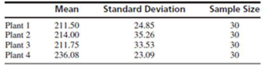
The article “Impact of Free Calcium Oxide Content of Fly Ash on Dust and Sulfur Dioxide Emissions in a Lignite-Fired Power Plant” (D. Sotiropoulos, A. Georgakopoulos, and N. Kolovos, Journal of Air and Waste Management, 2005:1042–1049) presents measurements of dust emissions, in mg/m3, for four power plants. Thirty measurements were taken for each plant. The sample means and standard deviations are presented in the following table:
- a. Construct an ANOVA table. You may give a
range for the P-value. - b. Can you conclude that there are differences among the
mean emission levels?
a.
Construct an ANOVA table and give a range for the P-value.
Answer to Problem 8E
The ANOVA table is,
| Source | DF | SS | MS | F | P |
| Plant | 3 | 12,712.7 | 4,237.6 | 4.8179 | 0.01<P-value<0.001 |
| Error | 116 | 102,027.8 | 879.55 | ||
| Total | 119 | 114,740.5 |
The range of P-value is
Explanation of Solution
Given info:
The data represents the means and standard deviations of 30 measurements of dust emissions taken on four types of plants.
Calculation:
The ANOVA table can be obtained as follows:
There are four samples, therefore
The total number of observations is,
The degrees of freedom corresponding to the plant is obtained as follows:
The degrees of freedom corresponding to the total is obtained as follows:
The degrees of freedom corresponding to the error is obtained as follows:
Total mean can be obtained as follows:
Substitute
The treatment sum of squares (SSTr) is obtained as follows:
Substitute
The error sum of squares (SSE) is obtained as follows:
Substitute
The total sum of squares (SST) is obtained as follows:
Substitute
The treatment mean square is obtained as follows:
Substitute
The error mean square is obtained as follows:
Substitute
The F-value is obtained as follows:
Substitute
Thus, the F-value is 4.8179.
From Appendix A table A.8, the upper 1% point of the
Therefore, the range of P-value is
Thus, the ANOVA table is,
| Source | DF | SS | MS | F | P |
| Plant | 3 | 12,712.7 | 4,237.6 | 4.8179 | 0.01<P-value<0.001 |
| Error | 116 | 102,027.8 | 879.55 | ||
| Total | 119 | 114,740.5 |
b.
Check whether the mean emission levels differ for four types of plants.
Answer to Problem 8E
There is sufficient evidence to conclude that the mean emission levels differ for four types of plants.
Explanation of Solution
Calculation:
State the hypotheses:
Null hypothesis:
Alternative hypothesis:
From part (a), the F-ratio is 4.8179.
P-value:
From part (a), the P-value is between 0.01 and 0.001.
Since, the level of significance is not specified; the prior level of significance
Decision:
If
If
Conclusion:
Here, the P-value is less than the level of significance.
That is,
By rejection rule, reject the null hypothesis.
There is sufficient evidence to conclude that the mean emission levels differ for four types of plants at
Want to see more full solutions like this?
Chapter 9 Solutions
Statistics for Engineers and Scientists
Additional Math Textbook Solutions
Basic Business Statistics, Student Value Edition (13th Edition)
Elementary Statistics (13th Edition)
Introductory Statistics
Statistics for Business and Economics (13th Edition)
Applied Statistics in Business and Economics


- A survey collected data on annual credit card charges in seven different categories of expenditures: transportation, groceries, dining out, household expenses, home furnishings, apparel, and entertainment. Using data from a sample of 42 credit card accounts, assume that each account was used to identify the annual credit card charges for groceries (population 1) and the annual credit card charges for dining out (population 2). Using the difference data, with population 1 − population 2, the sample mean difference was d = $870, and the sample standard deviation was sd = $1,124. (a) Formulate the null and alternative hypotheses to test for no difference between the population mean credit card charges for groceries and the population mean credit card charges for dining out. H0: ?d ≤ 0 Ha: ?d > 0 H0: ?d < 0 Ha: ?d = 0 H0: ?d ≥ 0 Ha: ?d < 0 H0: ?d = 0 Ha: ?d ≠ 0 H0: ?d ≠ 0 Ha: ?d = 0 (b) Calculate the test statistic. (Round your answer to three decimal…arrow_forwardThe article “Tibiofemoral Cartilage Thickness Distribution and its Correlation with Anthropometric Variables” (A. Connolly, D. FitzPatrick, et al., Journal of Engineering in Medicine, 2008:29–39) reports that in a sample of 11 men, the average volume of femoral cartilage (located in the knee) was 18.7 cm3 with a standard deviation of 3.3 cm3 and the average volume in a sample of 9 women was 11.2 cm3 with a standard deviation of 2.4 cm2. Find a 95% confidence interval for the difference in mean femoral cartilage volume between men and women.arrow_forwardNutritionResearchers compared protein intake among threegroups of postmenopausal women: (1) women eating astandard American diet (STD), (2) women eating a lactoovo-vegetarian diet (LAC), and (3) women eating a strictvegetarian diet (VEG). The mean ± 1 sd for protein intake(mg) is presented in Table 12.29.*12.1 Perform a statistical procedure to comparethe means of the three groups using the critical-valuemethod.arrow_forward
- In a study examining the effect of alcohol on reaction time, Liguori and Robinson (2001) found that even moderate alcohol consumption significantly slowed response time in a driving simulation. In a similar study, researchers measured the reaction time of a sample of n = 25 participants 30 minutes after drinking a 6-ounce glass of wine which ended up with a mean of = 422 millisecond. On the standardized driving simulation task, the population scores are normally distributed with a mean of µ = 400 millisecond with a standard deviation of σ = 40. Using an α = .05, conduct a hypothesis test to determine whether these data are sufficient to conclude that the alcohol significantly increased reaction time?arrow_forwardThe National Association of Home Builders provided data on the cost of the most popular home remodeling projects. Sample data on cost in thousands of dollars for two types if remodeling projects are as follows. Kitchen Master Bedroom 25.2 18.0 17.4 22.9 22.8 26.4 21.9 24.8 19.7 26.9 23.0 17.8 19.7 24.6 16.9 21.0 21.8 23.6 a. Compute the sample mean and sample standard deviation for each type of project. b. Develop a point estimate of the difference between the population mean…arrow_forwardRegular consumption of presweetened cereals con- tributes to tooth decay, heart disease, and other degen- erative diseases, according to studies conducted by Dr. W. H. Bowen of the National Institute of Health and Dr. J. Yudben, Professor of Nutrition and Dietetics at the University of London. In a random sample con- sisting of 20 similar single servings of Alpha-Bits, the average sugar content was 11.3 grams with a standard deviation of 2.45 grams. Assuming that the sugar con- tents are normally distributed, construct a 95% con- fidence interval for the mean sugar content for single servings of Alpha-Bits. Above and the number 9.9 attachment is the referred question of the 9.17 problemarrow_forward
 MATLAB: An Introduction with ApplicationsStatisticsISBN:9781119256830Author:Amos GilatPublisher:John Wiley & Sons Inc
 Probability and Statistics for Engineering and th...StatisticsISBN:9781305251809Author:Jay L. DevorePublisher:Cengage Learning
 Statistics for The Behavioral Sciences (MindTap C...StatisticsISBN:9781305504912Author:Frederick J Gravetter, Larry B. WallnauPublisher:Cengage Learning
 Elementary Statistics: Picturing the World (7th E...StatisticsISBN:9780134683416Author:Ron Larson, Betsy FarberPublisher:PEARSON
 The Basic Practice of StatisticsStatisticsISBN:9781319042578Author:David S. Moore, William I. Notz, Michael A. FlignerPublisher:W. H. Freeman
 Introduction to the Practice of StatisticsStatisticsISBN:9781319013387Author:David S. Moore, George P. McCabe, Bruce A. CraigPublisher:W. H. Freeman