
Videos
The article “Optimum Design of an A-pillar Trim with Rib Structures for Occupant Head Protection” (H. Kim and S. Kang. Proceedings of the Institution of Mechanical Engineers. 2001:1161–1169) discusses a study in which several types of A-pillars were compared to determine which provided the greatest protection to occupants of automobiles during a collision. Following is a one-way ANOVA table, where the treatments are three levels of longitudinal spacing of the rib (the article also discussed two insignificant factors, which are omitted here). There were nine replicates at each level. The response is the head injury criterion (HIC), which is a unitless quantity that measures the impact energy absorption of the pillar.

The treatment means were
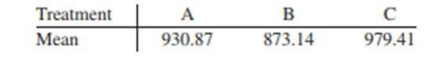
- a. Can you conclude that the longitudinal spacing affects the absorption of impact energy?
- b. Use the Tukey–Kramer method to determine which pairs of treatment means, if any. are different at the 5% level.
- c. Use the Bonferroni method to determine which pairs of treatment means, if any, are different at the 5% level.
- d. Which method is more powerful in this case, the Tukey-Kramer method or the Bonferroni method?

Trending nowThis is a popular solution!

Chapter 9 Solutions
Statistics for Engineers and Scientists
Additional Math Textbook Solutions
PRACTICE OF STATISTICS F/AP EXAM
Fundamentals of Statistics (5th Edition)
Elementary Statistics: Picturing the World (7th Edition)
Elementary Statistics ( 3rd International Edition ) Isbn:9781260092561
APPLIED STAT.IN BUS.+ECONOMICS
Business Statistics: A First Course (8th Edition)


- In a bumper test, three test vehicles of each of three types of autos were crashed into a barrier at 5 mph, and the resulting damage was estimated. Crashes were from three angles: head-on, slanted, and rear-end. The results are shown below. Research questions: Is the mean repair cost affected by crash type and/or vehicle type? Are the observed effects (if any) large enough to be of practical importance (as opposed to statistical significance)? 5 mph Collision Damage ($) Crash Type Goliath Varmint Weasel Head-On 700 1,700 2,280 1,400 1,650 1,670 850 1,630 1,740 Slant 1,430 1,850 2,000 1,740 1,700 1,510 1,240 1,650 2,480 Rear-end 700 860 1,650 1,250 1,550 1,650 970 1,250 1,240 (d) Perform Tukey multiple comparison tests. (Input the mean values within the input boxes of the first row and input boxes of the first column. Round your t-values and critical values to 2 decimal places and other answers to 1 decimal place.) Post hoc analysis for…arrow_forwardA statistical program is recommended. Jensen Tire & Auto is in the process of deciding whether to purchase a maintenance contract for its new computer wheel alignment and balancing machine. Managers feel that maintenance expense should be related to usage, and they collected the following information on weekly usage (hours) and annual maintenance expense (in hundreds of dollars). Weekly Usage(hours) AnnualMaintenanceExpense 13 17.0 10 22.0 20 30.0 28 37.0 32 47.0 17 30.5 24 32.5 31 39.0 40 51.5 38 40.0 #1) Develop the estimated regression equation that could be used to predict the annual maintenance expense (in hundreds of dollars) given the weekly usage (in hours). (Round your numerical values to two decimal places.) #2) The expected expense of a machine being used 34 hours per week is $ hundred.arrow_forwardThe National Transportation Safety Board wants to look at the safety of three different sizes of cars. Using the data below, determine the whether the mean pressure applied to the driver`s head during a crash is equal for each type of car at alpha = 0.01 Compact cars Midsize cars Full-size Cars 643 469 484 655 427 456 702 525 402 a) Ho: Ha : b) Decision c) Conclusionarrow_forward
- The table below shows the numbers of bushels of barley cultivated per acre for 12 one-acre plots of land for two different strains of barley, PHT-34 and CBX-21. PHT-34 CBX-21 43 55 49 46 47 43 38 44 47 45 45 49 50 47 46 59 46 52 46 49 45 48 43 51 Determine the minimum data value, the quartiles, and the maximum data value for the PHT-34 and CBX-21 data sets. PHT-34 CBX-21 min Q1 Q2 Q3 maxarrow_forwardNutritionResearchers compared protein intake among threegroups of postmenopausal women: (1) women eating astandard American diet (STD), (2) women eating a lactoovo-vegetarian diet (LAC), and (3) women eating a strictvegetarian diet (VEG). The mean ± 1 sd for protein intake(mg) is presented in Table 12.29. 12.5 Using the data in Table 12.29, perform a multiplecomparisons procedure to identify which specific underlyingmeans are different.arrow_forwardHigh levels of blood sugar are associated with an increased risk of type 2 diabetes. A levelhigher than normal is referred to as “impaired fasting glucose.” The article “Association ofLow-Moderate Arsenic Exposure and Arsenic Metabolism with Incident Diabetes andInsulin Resistance in the Strong Heart Family Study” (M. Grau-Perez, C. Kuo, et al.,Environmental Health Perspectives, 2017, online) reports a study in which 47 of 155 peoplewith impaired fasting glucose had type 2 diabetes. Consider this to be a simple randomsample. a) Find a 95% confidence interval for the proportion of people with impaired fasting glucose who have type 2 diabetes. b) Find a 99% confidence interval for the proportion of people with impaired fasting glucose who have type 2 diabetes. c) A doctor claims that less than 35% of people with impaired fasting glucose have type 2 diabetes. With what level of confidence can this claim be made?arrow_forward
- Since its removal from the banned substances list in 2004 by the World Anti-Doping Agency,caffeine has been used by athletes with the expectancy that it enhances their workout andperformance. However, few studies look at the role caffeine plays in sedentary females.Researchers at the University of Western Australia conducted a test in which they determined therate of energy expenditure (kilojoules) on 10 healthy, sedentary females who were nonregularcaffeine users. Each female was randomly assigned either a placebo or caffeine pill (6mg/kg) 60minutes prior to exercise. The subject rode an exercise bike for 15 minutes at 65% of theirmaximum heart rate, and the energy expenditure was measured. The process was repeated on aseparate day for the remaining treatment. The mean difference in energy expenditure (caffeine –placebo) was 18kJ with a standard deviation of 19kJ. If we assume that the differences follow anormal distribution can it be concluded that that caffeine appears to increase…arrow_forwardThe authors of the article “Predictive Model for PittingCorrosion in Buried Oil and Gas Pipelines”(Corrosion, 2009: 332–342) provided the data on whichtheir investigation was based.a. Consider the following sample of 61 observations onmaximum pitting depth (mm) of pipeline specimensburied in clay loam soil. 0.41 0.41 0.41 0.41 0.43 0.43 0.43 0.48 0.480.58 0.79 0.79 0.81 0.81 0.81 0.91 0.94 0.941.02 1.04 1.04 1.17 1.17 1.17 1.17 1.17 1.171.17 1.19 1.19 1.27 1.40 1.40 1.59 1.59 1.601.68 1.91 1.96 1.96 1.96 2.10 2.21 2.31 2.462.49 2.57 2.74 3.10 3.18 3.30 3.58 3.58 4.154.75 5.33 7.65 7.70 8.13 10.41 13.44Construct a stem-and-leaf display in which the twolargest values are shown in a last row labeled HI.b. Refer back to (a), and create a histogram based oneight classes with 0 as the lower limit of the firstclass and class widths of .5, .5, .5, .5, 1, 2, 5, and 5,respectively.c. The accompanying comparative boxplot fromMinitab shows plots of pitting depth for four differenttypes of soils.…arrow_forwardA market research company asked 9 people to evaluate a brand of tablet computer, Brand A, usinga questionnaire. The questionnaire scores are given in TABLE 1.TABLE 1Brand A 8.00 8.02 8.02 8.04. 8.04 8.04 8.07 8.10. 8.11 Another brand of tablet computer, Brand B, was evaluated and given scores with the informationas seen in TABLE 2.TABLE 2Information. Brand B. Minimum (min) 8.04First Quartile (Q1) 8.06Median (Q2) 8.07Third Quartile (Q3) 8.08Maximum (max) 8.10 a) Construct a boxplot for scores of Brand A and label it accordingly. b) Determine the interquartile range (IQR) for both brands.c) According to the IQRs in (b), which brand's scores were more varied in the evaluation? Why?arrow_forward
- On snow-covered roads, winter tires enable a car to stop in a shorter distance than if summer tires were installed. In terms of the additive model for one-way ANOVA, and for an experiment in which the mean stopping distances on a snow-covered road are measured for each of four brands of winter tires. If the data are as shown in Sheet 48, what conclusion would be reached at the 0.01 level of significance? Shett 48 Supplier A 517 484 463 452 502 447 481 500 485 566 Supplier B 479 499 488 430 482 457 424 488 526 455 Supplier C 435 443 480 465 435 430 465 514 463 510 Supplier D 526 537 443 505 468 533 481 477 490 470 Select one: a) p-value = 0.28 greater than 0.05, the average distance is different for at list two tires b) F stat = 1.86, F crit = 4.38, not enough evidence to claim that the average distance is different for at list two tires c) F ratio = 4.38, not enough evidence to claim that the average distance is different for at list two tires d) F stat = 0.68, F…arrow_forwardThe article “Wind-Uplift Capacity of Residential Wood Roof-Sheathing Panels Retrofitted with Insulating Foam Adhesive” (P. Datin, D. Prevatt, and W. Pang, Journal of Architectural Engineering, 2011:144–154) presents a study of the failure pressures of roof panels. Following are the failure pressures, in kPa, for five panels constructed with 6d smooth shank nails. These data are consistent with means and standard deviations presented in the article. 3.32 2.53 3.45 2.38 3.01 Find a 95% confidence interval for the mean failure pressure for this type of roof panel.arrow_forwardThree samples of each of three types of PVC pipe of equal wall thickness are tested to failure under three temperature conditions, yielding the results shown below. Research questions: Is mean burst strength affected by temperature and/or by pipe type? Is there a “best” brand of PVC pipe? Burst Strength of PVC Pipes (psi) Temperature PVC1 PVC2 PVC3 Hot (70º C) 247 299 239 277 287 262 283 275 279 Warm (40º C) 325 341 297 322 319 315 296 335 304 Cool (10º C) 358 375 327 366 352 334 338 359 340 Click here for the Excel Data File (a-1) Choose the correct row-effect hypotheses. a. H0: A1 ≠ A2 ≠ A3 ≠ 0 ⇐⇐ Temperature means differ H1: All the Aj are equal to zero ⇐⇐ Temperature means are the same b. H0: A1 = A2 = A3 = 0 ⇐⇐ Temperature means are the same H1: Not all the Aj are equal to zero ⇐⇐ Temperature means differ a b (a-2) Choose the correct column-effect hypotheses. a. H0: B1 ≠ B2 ≠ B3 ≠ 0 ⇐⇐…arrow_forward
 MATLAB: An Introduction with ApplicationsStatisticsISBN:9781119256830Author:Amos GilatPublisher:John Wiley & Sons Inc
 Probability and Statistics for Engineering and th...StatisticsISBN:9781305251809Author:Jay L. DevorePublisher:Cengage Learning
 Statistics for The Behavioral Sciences (MindTap C...StatisticsISBN:9781305504912Author:Frederick J Gravetter, Larry B. WallnauPublisher:Cengage Learning
 Elementary Statistics: Picturing the World (7th E...StatisticsISBN:9780134683416Author:Ron Larson, Betsy FarberPublisher:PEARSON
 The Basic Practice of StatisticsStatisticsISBN:9781319042578Author:David S. Moore, William I. Notz, Michael A. FlignerPublisher:W. H. Freeman
 Introduction to the Practice of StatisticsStatisticsISBN:9781319013387Author:David S. Moore, George P. McCabe, Bruce A. CraigPublisher:W. H. Freeman