
Videos
a.
Find the
a.
Answer to Problem 69SE
The 95% confidence interval for the slope of the population regression is
Explanation of Solution
Given info:
The data represents the values of the variables height in feet and price in dollars for a sample of warehouses.
Calculation:
Linear regression model:
In a linear equation
A linear regression model is given as
Regression:
Software procedure:
Step by step procedure to obtain regression equation using MINITAB software is given as,
- Choose Stat > Regression > Fit Regression Line.
- In Response (Y), enter the column of Price.
- In Predictor (X), enter the column of Height.
- Click OK.
Output using MINITAB software is given below:
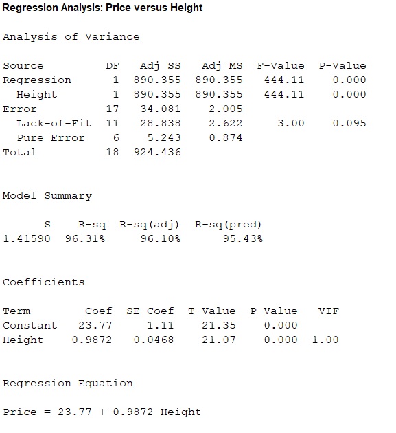
Thus, the regression line for the variables sale price
Therefore, the slope coefficient of the regression equation is
Confidence interval:
The general formula for the confidence interval for the slope of the regression line is,
Where,
From the MINITAB output, the estimate of error standard deviation of slope coefficient is
Since, the level of confidence is not specified. The prior confidence level 95% can be used.
Critical value:
For 95% confidence level,
Degrees of freedom:
The sample size is
The degrees of freedom is,
From Table A.5 of the t-distribution in Appendix A, the critical value corresponding to the right tail area 0.025 and 17 degrees of freedom is 2.110.
Thus, the critical value is
The 95% confidence interval is,
Thus, the 95% confidence interval for the slope of the population regression is
Interpretation:
There is 95% confident, that the expected change in sale price associated with 1 foot increase in height lies between $0.888452 and $1.085948.
c.
Find the interval estimate for the true
c.
Answer to Problem 69SE
The 95% specified confidence interval for the true mean sale price of all warehouses with 25 ft truss height is
Explanation of Solution
Calculation:
Here, the regression equation is
Expected sale price when the height is 25 feet:
The expected sale price with 25 ft height ware houses is obtained as follows:
Thus, the expected sale price with 25 ft height ware houses is 48.45.
Confidence interval:
The general formula for the
Where,
From the MINITAB output in part (a), the value of the standard error of the estimate is
The value of
| i | Truss height x | |
| 1 | 12 | 144 |
| 2 | 14 | 196 |
| 3 | 14 | 196 |
| 4 | 15 | 225 |
| 5 | 15 | 225 |
| 6 | 16 | 256 |
| 7 | 18 | 324 |
| 8 | 22 | 484 |
| 9 | 22 | 484 |
| 10 | 24 | 576 |
| 11 | 24 | 576 |
| 12 | 26 | 676 |
| 13 | 26 | 676 |
| 14 | 27 | 729 |
| 15 | 28 | 784 |
| 16 | 30 | 900 |
| 17 | 30 | 900 |
| 18 | 33 | 1089 |
| 19 | 36 | 1296 |
| Total |
Thus, the total of truss height is
The mean truss height is,
Thus, the mean truss height is
Covariance term
The value of
Thus, the covariance term
Since, the level of confidence is not specified. The prior confidence level 95% can be used.
Critical value:
For 95% confidence level,
Degrees of freedom:
The sample size is
The degrees of freedom is,
From Table A.5 of the t-distribution in Appendix A, the critical value corresponding to the right tail area 0.025 and 17 degrees of freedom is 2.110.
Thus, the critical value is
The 95% confidence interval is,
Thus, the 95% specified confidence interval for the true mean of all warehouses with 25 ft truss height is
Interpretation:
There is 95% specified confidence interval for the true mean of all warehouses with 25 ft truss height lies between $47.730 and $49.172.
d.
Find the prediction interval of sale price for a single warehouse of truss height 25 ft.
Compare the width of the prediction interval with the confidence interval obtained in part (a).
d.
Answer to Problem 69SE
The 95% prediction interval of sale price for a single warehouse of truss height 25 ft is
The prediction interval is wider than the confidence interval.
Explanation of Solution
Calculation:
Here, the regression equation is
From part (c), the the expected sale price with 25 ft height ware houses is
Prediction interval for a single future value:
Prediction interval is used to predict a single value of the focus variable that is to be observed at some future time. In other words it can be said that the prediction interval gives a single future value rather than estimating the mean value of the variable.
The general formula for
where
From the MINITAB output in part (a), the value of the standard error of the estimate is
From part (c), the truss height is
Since, the level of confidence is not specified. The prior confidence level 95% can be used.
Critical value:
For 95% confidence level,
Degrees of freedom:
The sample size is
The degrees of freedom is,
From Table A.5 of the t-distribution in Appendix A, the critical value corresponding to the right tail area 0.025 and 17 degrees of freedom is 2.110.
Thus, the critical value is
The 95% prediction interval is,
Thus, the 95% prediction interval of sale price for a single warehouse of truss height 25 ft is
Interpretation:
For repeated samples, there is 95% confident that the sale price for a single warehouse of truss height 25 ft lies between $45.377 and $51.523.
Comparison:
The 95% prediction interval of sale price for a single warehouse of truss height 25 ft is
Width of the prediction interval:
The width of the 95% prediction interval is,
Thus, the width of the 95% prediction interval is 6.146.
The 95% specified confidence interval for the true mean of all warehouses with 25 ft truss height is
Width of the confidence interval:
The width of the 95% confidence interval is,
Thus, the width of the 95% confidence interval is 1.442.
From, the obtained two widths it is observed that the width of the prediction interval is typically larger than the width of the confidence interval.
Thus, the prediction interval is wider than the confidence interval.
e.
Compare the width of the 95% prediction interval of sale price of ware houses for 25 ft truss height and for 30 ft truss height.
e.
Answer to Problem 69SE
The 95% prediction interval of sale price of ware houses for 30 ft truss height will be wider than the sale price of ware houses for 25 ft truss height.
Explanation of Solution
Calculation:
Here, the regression equation is
From part (c), the truss height is
Here, the observation
The general formula to obtain
For
For
In the two quantities, the only difference is the values of
In general, the value of the quantity
Therefore, the value
Comparison:
Prediction interval:
The general formula for
The prediction interval will be wider for large value of
Here,
Thus, the prediction interval is wider for
Thus, 95% prediction interval of sale price of ware houses for 30 ft truss height will be wider than the sale price of ware houses for 25 ft truss height.
e.
Find the
e.
Answer to Problem 69SE
The
Explanation of Solution
Calculation:
The coefficient of determination (
The general formula to obtain coefficient of variation is,
From the regression output obtained in part (a), the value of coefficient of determination is 0.9631.
Thus, the coefficient of determination is
Correlation coefficient:
Correlation analysis is used to measure the strength of the association between variables. In other words, it can be said that correlation describes the linear association between quantitative variables.
The general formula to calculate correlation coefficient is,
The coefficient of determination is obtained as follows:
The sign of the correlation coefficient depends on the sign of the slope coefficient.
Here,
Since, the sign of the slope coefficient is positive. The correlation coefficient is positive.
Thus, the correlation coefficient is 0.9814.
Interpretation:
The strength of the association between the variables sale price and truss height is 0.9814. that is, 1 unit increase in one variable is associated with 98.14% increase in the value of the other variable.
Want to see more full solutions like this?
Chapter 12 Solutions
Probability and Statistics for Engineering and the Sciences


- average heigth is 163 cm, standart deviation is 10 cm. compute p(X>168 cm) ?arrow_forwardThe average number of acres burned by forest and range fires in large new mexico country is 4,300 acres per year, with a standard debiation of 750 acre. The distribution of the number of acres burned is normal. What is the probabilty that between 2,500 and 4,200 acres will be burned in any given year?arrow_forwardNaini, Cobourne, McDonald and Donaldson (2008) reported that a specific ratio of height to face length of 1 to 8.5 tended to be rated as most attractive—almost exactly what Da Vinci’s idealized Vitruvian Man, predicts as “perfection” in the human form. For this study, we want to see if there is a relationship between a person’s height and head circumference. We get a random sample of 40 people and measure both their height and their head size to the nearest centimeter. What test should you use and why?arrow_forward
- Given that s.e.(b) = 61 and the estimate is 32, what is the t-stat?arrow_forwardIn forestry, the diameter of a tree at breast height is used to model the height of the tree. Silviculturists working in British Columbia’s boreal forest conducted a series of spacing trials to predict the heights of several species of trees. The data are the breast height diameters (in centimeters) and heights (in meters) for a sample of 18 white spruce trees. B1 B2 18.9 20.0 15.5 16.8 19.4 20.2 20.0 20.0 29.8 20.2 19.8 18.0 20.3 17.8 20.0 19.2 22.0 22.3 16.6 18.8 15.5 16.9 13.7 16.3 27.5 21.4 20.3 19.2 22.9 19.8 14.1 18.5 10.1 12.1 5.8 8.0 B1: Breast Height Diameter of White spruce (cm) B2: Height (m) a) Plot the relationship using scatter diagram between the breast height diameters and the trees’ height. Are the breast height diameters and the trees’ height linearly related? What can you infer about the relationship between the two variables? Is a linear model appropriate? b) Compare the scatter plot in (a) with the correlation coefficient…arrow_forwardA pharmaceutical company states that there is 500mg of active ingredient in each capsule for one of the medicines they manufacture. However, the FDA believes the company is purposely underfilling the capsule to save money. A sample of 20 capsules is taken and the amount of active ingredient inside is measured. The results are below: 484 460 471 512 494 529 494 485 474 502 503 538 466 495 475 529 518 464 449 489 Part 1: Construct a 95% confidence interval using toolPAK for the amount of active ingredient measured. Use the appropriate distribution, and specify the upper and lower limits of the interval. Part 2: Carefully interpret the 95% confidence interval? What if you did constructed a Confidence Interval Manually? Part 3: Does the 95% confidence interval support the FDA’s claim? Explain. Part 4: Would your answer change if the confidence level was lowered to 75%? Explain.arrow_forward
- Q1 A) List down the measures of central tendency and measures of dispersion 2) The operations manager of a plant that manufactures tires wants to compare the actual inner diameters of two grades of tires, each of B) which is expected to be 575 millimeters. A sample of five tires of each grade was selected, and the results representing the inner diameters of the tires, ranked from smallest to largest, are as follows. Grade X grade Y 568 570 575 578 584 573 574 575 577 578 requirement. a) for each of the tow grades of tries, compute the mwan, median, and standred deviation. b) which grade of tire providing better quality? explain. c) what would be the effect on your answer in (a) and (b) if the last value for grade Y were 588 insert 578 explain. C) The file contins the overall miles per gallon (MPG) OF 2010 family sedan: 24 21 22 23 24 34 34 34 20 20 22 22 44 32 20 20 22 20 39 20 Source:…arrow_forward(note: use mu for mean or average , p for proportion, >= for , <= for , =/ for ) State the null and alternative hypotheses to be used in testing the following claims and determine generally where the critical region is located: (a) The mean snowfall at Lake George during the month of February is 21.8 centimeters. Ho: Blank 1 H1: Blank 2 (b) No more than 20% of the faculty at the local university contributed to the annual giving fund. Ho: Blank 3 H1: Blank 4 (c) At least 70% of next year's new cars will be in the compact and subcompact category. Ho: Blank 5 H1: Blank 6 (d) The average rib-eye steak at the Longhorn Steak house is at least 340 grams. Ho: Blank 7 H1: Blank 8arrow_forwardTo assess the air quality in a surgical suite, the presence of colony-forming spores per cubic meter of air is measured on three successive days. The results are as follows: {12, 24, 30}. Calculate the mean and standard deviation for these data.arrow_forward
- C.2 A consumer group is interested in estimating the proportion of packages of ground beef sold at a particular store that have an actual fat content exceeding the fat content stated on the label. How many packages of ground beef should be tested to estimate this proportion to within .05 with 95% confidence?arrow_forwardThe mean yield from process A is estimated to be 80 ± 5, where the units are percent of a theoretical maximum. The mean yield from process B is estimated to be 90 ± 3. The relative increase obtained from process B is therefore estimated to be (90 − 80)/80 = 0.125. Find the uncertainty in this estimate.arrow_forwardUse the given information to find the minimum sample size required to estimate an unknown population mean How many weeks of data must be randomly sampled to estimate the mean weekly sales of a new line of athletic footwear? We want 98% confidence that the sample mean is within $500 of the population mean, and the population standard deviation is known to be $1500.arrow_forward
 MATLAB: An Introduction with ApplicationsStatisticsISBN:9781119256830Author:Amos GilatPublisher:John Wiley & Sons Inc
 Probability and Statistics for Engineering and th...StatisticsISBN:9781305251809Author:Jay L. DevorePublisher:Cengage Learning
 Statistics for The Behavioral Sciences (MindTap C...StatisticsISBN:9781305504912Author:Frederick J Gravetter, Larry B. WallnauPublisher:Cengage Learning
 Elementary Statistics: Picturing the World (7th E...StatisticsISBN:9780134683416Author:Ron Larson, Betsy FarberPublisher:PEARSON
 The Basic Practice of StatisticsStatisticsISBN:9781319042578Author:David S. Moore, William I. Notz, Michael A. FlignerPublisher:W. H. Freeman
 Introduction to the Practice of StatisticsStatisticsISBN:9781319013387Author:David S. Moore, George P. McCabe, Bruce A. CraigPublisher:W. H. Freeman