
Introduction To Statistics And Data Analysis
6th Edition
ISBN: 9781337793612
Author: PECK, Roxy.
Publisher: Cengage Learning,
expand_more
expand_more
format_list_bulleted
Videos
Textbook Question
Chapter 16.3, Problem 21E
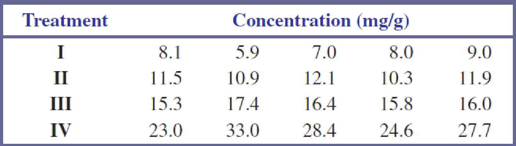
The given data on phosphorus concentration in topsoil for four different soil treatments appeared in the article “Fertilisers for Lotus and Clover Establishments on a Sequence of Acid Soils on the East Otago Uplands” (New Zealand Journal of Experimental Agriculture [1984]: 119–129).
Use the KW test and a 0.01 significance level to test the null hypothesis of no difference in true
Expert Solution & Answer

Trending nowThis is a popular solution!

Students have asked these similar questions
On snow-covered roads, winter tires enable a car to stop in a shorter distance than if summer tires were installed. In terms of the additive model for one-way ANOVA, and for an experiment in which the mean stopping distances on a snow-covered road are measured for each of four brands of winter tires. If the data are as shown in Sheet 48, what conclusion would be reached at the 0.01 level of significance?
Shett 48
Supplier A
517
484
463
452
502
447
481
500
485
566
Supplier B
479
499
488
430
482
457
424
488
526
455
Supplier C
435
443
480
465
435
430
465
514
463
510
Supplier D
526
537
443
505
468
533
481
477
490
470
Select one:
a) p-value = 0.28 greater than 0.05, the average distance is different for at list two tires
b) F stat = 1.86, F crit = 4.38, not enough evidence to claim that the average distance is different for at list two tires
c) F ratio = 4.38, not enough evidence to claim that the average distance is different for at list two tires
d) F stat = 0.68, F…
In analyzing the consumption of cottage cheese by members of various occupational groups, the United Dairy Industry Association found that 326 of 837 professionals seldom or never ate cottage cheese, versus 220 of 489 white-collar workers and 522 of 1243 blue-collar workers (Sheet 53). Assuming independent samples, use the 0.03 level in testing the null hypothesis that the population proportions could be the same for the three occupational groups.
Sheet 53
Group 1
Group 2
Group 3
Total
seldom or never
326
220
522
1068
often
511
269
721
1501
Total
837
489
1243
2569
Select one:
a) chi-square stat = 4.81, crit. value = 7.01, fail to reject H0, population proportions are not different
b) p-value = 0.09, reject H0, population proportions are not different
c) chi-square stat = 4.81, crit. value = 9.2, fail to reject H0, population proportions are not different
d) p-value = 0.029, reject H0, population proportions different
A Canadian study measuring depression level in teens (as reported in the Journal of Adolescence, vol. 25, 2002) randomly sampled 112 male teens and 101 female teens, and scored them on a common depression scale (higher score representing more depression). The researchers suspected that the mean depression score for male teens is higher than for female teens, and wanted to check whether data would support this hypothesis.
If μ1 and μ2 represent the mean depression score for male teens and female teens respectively, which of the following is an appropriate pair of hypotheses in this case? Check all that apply.
Chapter 16 Solutions
Introduction To Statistics And Data Analysis
Ch. 16.1 - Urinary fluoride concentration (in parts per...Ch. 16.1 - Prob. 2ECh. 16.1 - Prob. 3ECh. 16.1 - A blood lead level of 70 mg/ml has been commonly...Ch. 16.1 - The effectiveness of antidepressants in treating...Ch. 16.1 - Prob. 6ECh. 16.1 - Prob. 7ECh. 16.2 - The effect of a restricted diet in the treatment...Ch. 16.2 - Peak force (N) on the hand was measured just prior...Ch. 16.2 - In an experiment to study the way in which...
Ch. 16.2 - Prob. 11ECh. 16.2 - Prob. 12ECh. 16.2 - Prob. 13ECh. 16.2 - Prob. 14ECh. 16.2 - Prob. 15ECh. 16.2 - Prob. 16ECh. 16.2 - Prob. 17ECh. 16.2 - The signed-rank test can be adapted for use in...Ch. 16.3 - Prob. 19ECh. 16.3 - Prob. 20ECh. 16.3 - The given data on phosphorus concentration in...Ch. 16.3 - Prob. 22ECh. 16.3 - Prob. 23ECh. 16.3 - The following data on amount of food consumed (g)...Ch. 16.3 - The article Effect of Storage Temperature on the...
Knowledge Booster


Learn more about
Need a deep-dive on the concept behind this application? Look no further. Learn more about this topic, statistics and related others by exploring similar questions and additional content below.Similar questions
- From a sample of 14 observations, an analyst calculates a t-statistic to test a hypothesis that the population mean is equal to zero. If the analyst chooses a 5% significance level, the appropriate critical value is: A. less than 1.80. B. greater than 2.16. C. between 1.80 and 2.16.arrow_forwardA simple random sample of front-seat occupants involved in car crashes is obtained. Among3000occupants not wearing seat belts,36were killed. Among 7697occupants wearing seat belts,18were killed. Use a0.05significance level to test the claim that seat belts are effective in reducing fatalities. Complete parts (a) through (c) below.arrow_forwardThe number of contaminating particles on a silicon waferprior to a certain rinsing process was determined for eachwafer in a sample of size 100, resulting in the followingfrequencies:Number of particles 0 1 2 3 4 5 6 7Frequency 1 2 3 12 11 15 18 10Number of particles 8 9 10 11 12 13 14Frequency 12 4 5 3 1 2 1a. What proportion of the sampled wafers had at leastone particle? At least five particles?b. What proportion of the sampled wafers had betweenfive and ten particles, inclusive? Strictly between fiveand ten particles?c. Draw a histogram using relative frequency on thevertical axis. How would you describe the shape of thehistogram?arrow_forward
- NutritionResearchers compared protein intake among threegroups of postmenopausal women: (1) women eating astandard American diet (STD), (2) women eating a lactoovo-vegetarian diet (LAC), and (3) women eating a strictvegetarian diet (VEG). The mean ± 1 sd for protein intake(mg) is presented in Table 12.29. 12.5 Using the data in Table 12.29, perform a multiplecomparisons procedure to identify which specific underlyingmeans are different.arrow_forwardThe authors of the article “Predictive Model for PittingCorrosion in Buried Oil and Gas Pipelines”(Corrosion, 2009: 332–342) provided the data on whichtheir investigation was based.a. Consider the following sample of 61 observations onmaximum pitting depth (mm) of pipeline specimensburied in clay loam soil. 0.41 0.41 0.41 0.41 0.43 0.43 0.43 0.48 0.480.58 0.79 0.79 0.81 0.81 0.81 0.91 0.94 0.941.02 1.04 1.04 1.17 1.17 1.17 1.17 1.17 1.171.17 1.19 1.19 1.27 1.40 1.40 1.59 1.59 1.601.68 1.91 1.96 1.96 1.96 2.10 2.21 2.31 2.462.49 2.57 2.74 3.10 3.18 3.30 3.58 3.58 4.154.75 5.33 7.65 7.70 8.13 10.41 13.44Construct a stem-and-leaf display in which the twolargest values are shown in a last row labeled HI.b. Refer back to (a), and create a histogram based oneight classes with 0 as the lower limit of the firstclass and class widths of .5, .5, .5, .5, 1, 2, 5, and 5,respectively.c. The accompanying comparative boxplot fromMinitab shows plots of pitting depth for four differenttypes of soils.…arrow_forwardThe NAEP considers that a national average of 283 is an acceptable performance. Using α = .05, run a two-tail t-test for one sample to test Ho: µ=283 for the 2019 scores. Report the t-obt, df, and p-values. Would you reject the null hypothesis that the 2019 scores come from a population with average 283? If this is the case, does it come from a population from larger or smaller average?arrow_forward
- When companies are designing a new product, one of the steps typically taken is to see how potential buyers react to a picture or prototype of the proposed product. The product-development team for a notebook computer company has shown picture A to a large sample of potential buyers and picture B to another, asking each person to indicate what they "would expect to pay" for such a product. The data resulting from the two pictures are provided in file (sheet 6). Using the 0.05 level of significance, determine whether the prototypes might not really differ in terms of the price that potential buyers would expect to pay. Sheet 6 ComputerA ComputerB 3 317 2 965 2 680 3 083 3 286 3 137 2 859 2 950 2 693 3 161 2 945 2 918 2 908 3 158 3 193 3 082 3 240 2 903 3 040 3 103…arrow_forwardBased on a survey of a random sample of 900 adults in the United States, a journalist reports that A random sample of 100 movie goers was asked to state his or her gender and favorite soft drink available at the local movie theater. The results appear in the table below. Is there a relationship between gender and soft drink preference? Coke Diet Coke Sprite Male 23 11 12 Female 16 28 10 To analyze the results, which of the following tests is most appropriate? A)Chi-square test of independence B)Chi-square test of homogeneity C)Two sample t-test D)Matched pair t-test E)Chi-square goodness of fitarrow_forwardThree samples of each of three types of PVC pipe of equal wall thickness are tested to failure under three temperature conditions, yielding the results shown below. Research questions: Is mean burst strength affected by temperature and/or by pipe type? Is there a “best” brand of PVC pipe? Burst Strength of PVC Pipes (psi) Temperature PVC1 PVC2 PVC3 Hot (70º C) 247 299 239 277 287 262 283 275 279 Warm (40º C) 325 341 297 322 319 315 296 335 304 Cool (10º C) 358 375 327 366 352 334 338 359 340 Click here for the Excel Data File (a-1) Choose the correct row-effect hypotheses. a. H0: A1 ≠ A2 ≠ A3 ≠ 0 ⇐⇐ Temperature means differ H1: All the Aj are equal to zero ⇐⇐ Temperature means are the same b. H0: A1 = A2 = A3 = 0 ⇐⇐ Temperature means are the same H1: Not all the Aj are equal to zero ⇐⇐ Temperature means differ a b (a-2) Choose the correct column-effect hypotheses. a. H0: B1 ≠ B2 ≠ B3 ≠ 0 ⇐⇐…arrow_forward
arrow_back_ios
arrow_forward_ios
Recommended textbooks for you
 MATLAB: An Introduction with ApplicationsStatisticsISBN:9781119256830Author:Amos GilatPublisher:John Wiley & Sons Inc
 Probability and Statistics for Engineering and th...StatisticsISBN:9781305251809Author:Jay L. DevorePublisher:Cengage Learning
 Statistics for The Behavioral Sciences (MindTap C...StatisticsISBN:9781305504912Author:Frederick J Gravetter, Larry B. WallnauPublisher:Cengage Learning
 Elementary Statistics: Picturing the World (7th E...StatisticsISBN:9780134683416Author:Ron Larson, Betsy FarberPublisher:PEARSON
 The Basic Practice of StatisticsStatisticsISBN:9781319042578Author:David S. Moore, William I. Notz, Michael A. FlignerPublisher:W. H. Freeman
 Introduction to the Practice of StatisticsStatisticsISBN:9781319013387Author:David S. Moore, George P. McCabe, Bruce A. CraigPublisher:W. H. Freeman
MATLAB: An Introduction with Applications
Statistics
ISBN:9781119256830
Author:Amos Gilat
Publisher:John Wiley & Sons Inc
Probability and Statistics for Engineering and th...
Statistics
ISBN:9781305251809
Author:Jay L. Devore
Publisher:Cengage Learning
Statistics for The Behavioral Sciences (MindTap C...
Statistics
ISBN:9781305504912
Author:Frederick J Gravetter, Larry B. Wallnau
Publisher:Cengage Learning
Elementary Statistics: Picturing the World (7th E...
Statistics
ISBN:9780134683416
Author:Ron Larson, Betsy Farber
Publisher:PEARSON
The Basic Practice of Statistics
Statistics
ISBN:9781319042578
Author:David S. Moore, William I. Notz, Michael A. Fligner
Publisher:W. H. Freeman
Introduction to the Practice of Statistics
Statistics
ISBN:9781319013387
Author:David S. Moore, George P. McCabe, Bruce A. Craig
Publisher:W. H. Freeman
Introduction to experimental design and analysis of variance (ANOVA); Author: Dr. Bharatendra Rai;https://www.youtube.com/watch?v=vSFo1MwLoxU;License: Standard YouTube License, CC-BY