Videos
An accurate assessment of oxygen consumption provides important information for determining energy expenditure requirements for physically demanding tasks. The paper “Oxygen Consumption During Fire Suppression: Error of Heart Rate Estimation” (Ergonomics [1991]: 1469–1474) reported on a study in which x = Oxygen consumption (in milliliters per kilogram per minute) during a treadmill test was determined for a sample of 10 firefighters. Then y = Oxygen consumption at a comparable heart rate was measured for each of the 10 individuals while they performed a fire-suppression simulation. This resulted in the following data and

- a. Does the scatterplot suggest an approximate linear relationship?
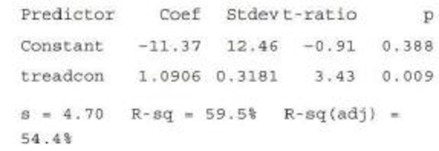
- b. The investigators fit a least-squares line. The resulting Minitab output is given in the following:
The regression equation is firecon = 211. 4 + 1. 09 treadcon
Predict fire-simulation consumption when treadmill consumption is 40.
- c. How effectively does a straight line summarize the relationship?
- d. Delete the first observation, (51.3, 49.3), and calculate the new equation of the least-squares line and the value of r2. What do you conclude? (Hint: For the original data, Σx = 388.8, Σy = 310 .3, Σx2 = 15,338.54, Σxy = 12,306.58, and Σy2 = 10,072.41.)
a.
Discuss whether the scatterplot indicates an approximate linear relationship.
Answer to Problem 66CR
No, the scatterplot does not indicate an approximate linear relationship.
Explanation of Solution
The data relates the oxygen consumption (milliliters per kilogram per minute) of 10 firefighters during a fire-suppression simulation, y to that during a treadmill test, x. The scatterplot between the two variables is given.
Denote the estimated response variable as
A careful inspection of the given scatterplot shows that the points do not fall on a straight line. Rather, the points are scattered almost in a random manner, without showing any pattern in particular. However, there is one extreme point, which is far away from the remaining points. This extreme point appears to provide an impression that there might be a linear relationship between the two variables. Once this point is ignored, it is clear that no such relationship can be determined.
Thus, the scatterplot does not indicate an approximate linear relationship.
b.
Predict the fire-simulation oxygen consumption, if the treadmill oxygen consumption is 40.
Answer to Problem 66CR
The fire-simulation oxygen consumption, when the treadmill oxygen consumption is 40 is 32.254 milliliters per kilogram per minute.
Explanation of Solution
Calculation:
The MINITAB output for the fitting of a least-squares regression line to the given data is given.
In the given output, the column of “Coef” gives the coefficients corresponding to the variables given in the column of “Predictor”. The term “Constant” under the column of ‘Predictor’ gives the intercept of the equation; the term “treadcon” denotes the oxygen consumption of during the treadmill test, x.
Using the values in the output, the equation of the least-squares regression line is
For a treadmill oxygen consumption of 40 milliliters per kilogram per minute,
Thus, the fire-simulation oxygen consumption, when the treadmill oxygen consumption is 40 is 32.254 milliliters per kilogram per minute.
c.
Explain the effectivity of the straight line to summarize the relationship between the variables.
Explanation of Solution
In the given output, the value of
Now,
Thus, it can be interpreted that the oxygen consumption during the treadmill test can predict about 59.5% of the variability in the oxygen consumption during the fire-suppression simulation.
This suggests that the straight line is moderately effective in summarizing the relationship between the variables.
d.
Find the equation of the least-squares line and the value of
Answer to Problem 66CR
The equation of the least-squares line after deleting the first observation, (51.3, 49.3) is
The value of
Explanation of Solution
Calculation:
It is given that, for the original data set,
For the first observation,
Now, the lest-squares regression line is of the form:
Using this formula and the values obtained above, b and a are respectively obtained as follows:
Now,
Thus,
Using the values of a and b obtained above, the equation of the least-squares line after deleting the first observation, (51.3, 49.3) is
Now, it is known that the slope for the least-squares regression of y on x, that is, b can be given by the formula:
Now, it can be shown that:
Similarly,
Thus,
Using the values obtained above, the value of r can be calculated as follows:
It is known that
Hence, the value of
Now,
Now,
Thus, it can be interpreted that the oxygen consumption during the treadmill test can predict about 2% of the variability in the oxygen consumption during the fire-suppression simulation, which is a very low percentage.
Thus, the model 9is not a very good fit for the data.
Want to see more full solutions like this?
Chapter 5 Solutions
Bundle: Introduction to Statistics and Data Analysis, 5th + WebAssign Printed Access Card: Peck/Olsen/Devore. 5th Edition, Single-Term
Additional Math Textbook Solutions
Statistics for Business & Economics, Revised (MindTap Course List)
Elementary Statistics
Basic Business Statistics, Student Value Edition
Introductory Statistics (2nd Edition)
Elementary Statistics: A Step By Step Approach
Essentials of Statistics, Books a la Carte Edition (5th Edition)


- The paper "Accelerated Telomere Shortening in Response to Life Stress" (Proceedings of the National Academy of Sciences (2004): 17312-17315) described a study that examined whether stress accelerates aging at a cellular level. The accompanying data on a measure of perceived stress (x) and telomere length (y) were read from a scatterplot that appeared in the paper. Telomere length is a measure of cell longevity. 5.38 Perceived Telomere Perceived Telomere Stress Length Stress Length 5 1.25 20 1.22 1.32 20 1.30 1.5 20 1.32 7 1.35 21 1.24 10 1.3 21 1.26 11 1 21 1.30 12 1.18 22 1.18 13 1.1 22 1.22 14 1.08 22 1.24 14 1.3 23 1.18 15 0.92 24 1.12 15 1.22 24 1.50 15 1.24 25 0.94 17 1.12 26 0.84 17 1.32 27 1.02 17 1.4 27 1.12 18 1.12 28 1.22 18 1.46 29 1.30 19 0.84 33 0.94 a. Compute the equation of the least-squares line. b. What is the value of r? c. Does the linear relationship between perceived stress and telomere length account for a large or small proportion of the variability in telomere…arrow_forwardA study was conducted to examine the effect of diet cola consumption on calcium levels in women. A sample of 16 healthy women aged 18 to 40 were randomly assigned to drink 24 ounces of either diet cola or water. Their urine was collected for three hours after ingestion of the beverage and calcium excretion (in mg) was measured. The data are stored in ColaCalcium.arrow_forwardThe removal of ammoniacal nitrogen is an important aspect of treatment of leachate at landfill sites. The rate of removal (in percent per day) is recorded for several days for each of several treatment methods. The results are presented in the following table. (Based on the article "Removal of Ammoniacal Nitrogen from Landfill Leachate by Irrigation onto Vegetated Treatment Planes," S. Tyrrel, P. Leeds-Harrison, and K. Harrison, Water Research, 2002:291–299.) Treatment Rate of Removal 5.21 4.65 5.59 2.69 7.57 5.16 6.24 5.94 6.41 6.85 9.18 4.94 4.04 3.29 4.52 3.75 Construct an ANOVA table. You may give a range for the P-value. Can you conclude that the treatment methods differ in their rates of removal? a. b. ABCAEarrow_forward
- A deficiency of the trace element selenium in the diet can negatively impact growth, immunity, muscle and neuromuscular function, and fertility. The introduction of selenium supplements to dairy cows is justified when pastures have low selenium levels. Authors of a research paper supplied the following data on milk selenium concentration (mg/L) for a sample of cows given a selenium supplement (the treatment group) and a control sample given no supplement, both initially and after a 9-day period. Initial Measurement Treatment Control 11.4 9.1 9.6 8.7 10.1 9.7 8.5 10.8 10.2 10.9 10.6 10.6 11.9 10.1 9.9 12.3 10.7 8.8 10.2 10.4 10.3 10.9 11.4 10.4 9.3 11.6 10.6 10.9 10.9 8.3 After 9 Days Treatment Control 138.3 9.2 104 8.9 96.4 8.9 89 10.1 88 9.6 103.8 8.6 147.3 10.4 97.1 12.4 172.6 9.2 146.3 9.5 99 8.4 122.3 8.8 103 12.5 117.8 9.1 121.5 93 (a) Use the given data for the treatment group to determine if…arrow_forwardA deficiency of the trace element selenium in the diet can negatively impact growth, immunity, muscle and neuromuscular function, and fertility. The introduction of selenium supplements to dairy cows is justified when pastures have low selenium levels. Authors of a research paper supplied the following data on milk selenium concentration (mg/L) for a sample of cows given a selenium supplement (the treatment group) and a control sample given no supplement, both initially and after a 9-day period. Initial Measurement Treatment Control 11.2 9.1 9.6 8.7 10.1 9.7 8.5 10.8 10.3 10.9 10.6 10.6 11.7 10.1 9.7 12.3 10.8 8.8 10.3 10.4 10.4 10.9 11.2 10.4 9.4 11.6 10.6 10.9 10.7 8.4 After 9 Days Treatment Control 138.3 9.3 104 8.7 96.4 8.7 89 10.1 88 9.6 103.8 8.6 147.3 10.2 97.1 12.2 172.6 9.3 146.3 9.5 99 8.2 122.3 8.9 103 12.5 117.8 9.1 121.5 93 (a) Use the given data for the treatment group to determine if there…arrow_forwardA deficiency of the trace element selenium in the diet can negatively impact growth, immunity, muscle and neuromuscular function, and fertility. The introduction of selenium supplements to dairy cows is justified when pastures have low selenium levels. Authors of a research paper supplied the following data on milk selenium concentration (mg/L) for a sample of cows given a selenium supplement (the treatment group) and a control sample given no supplement, both initially and after a 9-day period. Initial Measurement Treatment Control 11.3 9.1 9.7 8.7 10.1 9.7 8.5 10.8 10.4 10.9 10.7 10.6 11.8 10.1 9.8 12.3 10.6 8.8 10.4 10.4 10.2 10.9 11.3 10.4 9.2 11.6 10.7 10.9 10.8 8.2 After 9 Days Treatment Control 138.3 9.4 104 8.8 96.4 8.8 89 10.1 88 9.7 103.8 8.7 147.3 10.3 97.1 12.3 172.6 9.4 146.3 9.5 99 8.3 122.3 8.9 103 12.5 117.8 9.1 121.5 93 (a) Use the given data for the treatment group to determine if…arrow_forward
- Are seatbelts effective at saving lives? We wish to examine whether or not the use of seatbelts reduces fatalities at the a = 0.01 level of significance. Let pN represent the proportion of non-seatbelt wearing passengers who were involved in a crash and died and py represent the proportion of seatbelt wearing passengers who were involved in a crash and died. NOTE: The data used in this study were obtained through observational study...no experiment was conducted! Which would be correct hypotheses for this test? O Ho:PN = pY, H1:PN > pY Ho: PN = pY, H,:PN Py In a random sample of 321 non-seatbelt wearing passengers involved in a car crash, 30 were killed. In a random sample of 492 seatbelt wearing passengers involved in a car crash, 13 were killed. Find the test statistic (2 decimal places): Give the P-value (4 decimal places - if less than 0.001 answer 0): Which is the correct result: Reject the Null Hypothesis O Do not Reject the Null Hypothesis Which would be the appropriate…arrow_forwardThe depth of wetting of a soil is the depth to which water content will increase owing to extemal factors. The article "Discussion of Method for Evaluation of Depth of Wetting in Residential Areas" (J. Nelson, K. Chao, and D. Overton, Journal of Geotechnical and Geoenvironmental Engineering, 2011:293-296) discusses the relationship between depth of wetting beneath a structure and the age of the structure. The article presents measurements of depth of wetting, in meters, and the ages, in years, of 21 houses, as shown in the following table. Age Depth 7.6 4 4.6 6.1 9.1 3 4.3 7.3 5.2 10.4 15.5 5.8 10.7 4 5.5 6.1 10.7 10.4 4.6 7.0 6.1 14 16.8 10 9.1 8.8 Compute the least-squares line for predicting depth of wetting (y) from age (x). b. Identify a point with an unusually large x-value. Compute the least-squares line that results from deletion of this point. Identify another point which can be classified as an outlier. Compute the least-squares line that results from deletion of the outlier,…arrow_forwardEstriol Level and Birth Weight. J. Greene and J. Touchstone conducted a study on the relationship between the estriol levels of pregnant women and the birth weights of their children. Their findings, “Urinary Tract Estriol: An Index of Placental Function,” were published in the American Journal of Obstetrics and Gynecology (Vol. 85(1), pp. 1–9). The data from the study are provided on the WeissStats site, where estriol levels are in mg/24 hr and birth weights are in hectograms. a. Decide whether finding a regression line for the data is reasonable. If so, then also do parts (b)–(d). b. Obtain the coefficient of determination. c. Determine the percentage of variation in the observed values of the response variable explained by the regression, and interpret your answer. d. State how useful the regression equation appears to be for making predictions.arrow_forward
- A methodological study had established values for the MIC on a scale that measured physical function: The MIC for improvement (higher scores) was 4.0, and the MIC for deterioration (lower scores) was 3.0. Lawrence studied clinically significant change in physical functioning over a 1-year period for a sample of 100 patients with COPD. Some change score information is presented below for 10 patients. Which patients experienced clinically significant change in physical function in the 12-month period between assessments? Patient Baseline Score* 12-Month Score* 1 19 15 2 12 10 3 16 14 4 17 16 5 9 10 6 11 12 7 13 17 8 15 13 9 18 14 10 16 9 *Higher scores = higher level of physical function Which patients had clinically significant deterioration? Which patients had clinically significant improvement? Which patients had no clinically significant change?arrow_forwardAn article in the Journal of Environmental Engineering (1989, Vol. 115(3), pp. 608–619) reported the results of a study on the occurrence of sodium and chloride in surface streams in central Rhode Island. The following data are chloride concentration y (in milligrams per liter) and roadway area in the watershed x (in percentage).arrow_forwardA study published by Babcock and Marks (2010) showed that the average full-time U.S. college student studied for μ = 14 hours per week (SD = 4.8 hours per week) in 2005. We want to know if this average has changed in the past 15 years. In other words, we are going to do a study in which we try to determine whether there has been an impact of the passage of time on the amount of time college students spend studying. We selected a sample of n = 64 of today’s college students and find that they spent an average of M = 12.5 hours per week studying. Does this sample indicate a significant change in the number of hours spent studying? Use a two-tailed test (this means non-directional hypothesis) with α = .05.arrow_forward
 Calculus For The Life SciencesCalculusISBN:9780321964038Author:GREENWELL, Raymond N., RITCHEY, Nathan P., Lial, Margaret L.Publisher:Pearson Addison Wesley,
 Glencoe Algebra 1, Student Edition, 9780079039897...AlgebraISBN:9780079039897Author:CarterPublisher:McGraw Hill