
Videos
(a)
To graph: The histogram.
(a)
Explanation of Solution
Calculation:
To draw the histogram, follow the below mentioned steps in Minitab:
Step 1: Enter the data in Minitab and enter variable name as “Diameter.”
Step 2: Go to “Graph” and point on “Histogram.” Click on “Simple” and then press OK.
Step 3: In dialog box that appears, select “Diameter” under the field marked as “Graph variable,” and then click on OK.
The histogram obtained is as follows:
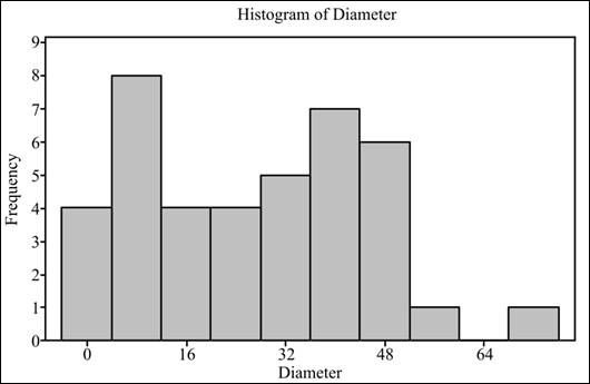
Interpretation: The histogram does not seem to represent a bell-shaped curve.
To graph: The box plot.
Explanation of Solution
Graph: To draw the box plot, follow the below mentioned steps in Minitab:
Step 1: Enter the data in Minitab and enter variable name as “Diameter.”
Step 2: Go to
Step 3: In dialog box that appears, select “Diameter” under the field marked as “Graph variable,” and then click on OK.
The required box plot is as follows:
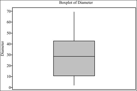
Interpretation: From the box plot, the data does not appear to be symmetrical.
To graph: The normal quantile plot.
Explanation of Solution
Given: The data for the diameters of 40 randomly sampled trees is provided.
Calculation: To draw the normal quantile plot, follow the below mentioned steps in SPSS.
Step 1: Enter the data of diameter in SPSS and enter the variable name “Diameter.”
Step 2: Go to
Step 3: Select “Diameter” under the field marked as “Variables.” Finally, click on “Ok.”
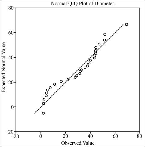
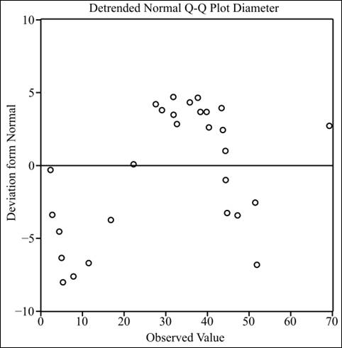
The normal quantile plots are as follows:
To explain: The distribution.
Answer to Problem 33E
Solution: The distribution is not normal as it has two peaks, and the normal quantile plot shows that the distribution is deviated from the
Explanation of Solution
The histogram of the distribution shows that it has two peaks. In the box plot, the upper tail is longer than the lower tail, which indicates its deviation from normality, and the normal quantile plots also show that the data is deviated from the normal distribution as most of the values are away from the normal position.
(b)
Whether t procedures can be used to calculate 95% confidence interval.
(b)
Answer to Problem 33E
Solution: The t procedures can be used as the sample is large enough to eliminate the effect of non-normal distribution.
Explanation of Solution
As the data is large enough as compared to the population, it will eliminate the effect of non-normality. So, the t procedures can be used.
(c)
Section 1:
To find: The margin of error.
(c)
Section 1:
Answer to Problem 33E
Solution: The margin of error is 5.68.
Explanation of Solution
Calculation:
To calculate the margin of error, first, standard deviation and mean of the sample need to be calculated. To calculate standard deviation and mean, follow the below mentioned steps in Minitab:
Step 1: Enter the data in Minitab and enter variable name as “Diameter.”
Step 2: Go to
Step 3: In dialog box that appears, select “Diameter” under the field marked as “Variables,” and then click on “Statistics.”
Step 4: In dialog box that appears, select “None” and then “Mean” and “Standard deviation.” Finally, click on “Ok” on both dialog boxes.
From Minitab result, the standard deviation is 17.71 and the mean is 27.29.
The formula for margin of error is as follows:
where
Section 2:
To find: The 95% confidence interval for mean diameter.
Section 2:
Answer to Problem 33E
Solution: The 95% confidence interval is
Explanation of Solution
Calculation:
The confidence interval is an interval for which there are 95% chances that it contains the population parameter (population mean).
To calculate confidence interval, follow the below mentioned steps in Minitab:
Step 1: Enter the provided data into Minitab and enter variable name as “Diameter.”
Step 2: Go to
Step 3: In the dialog box that appears, select “Diameter” under the field marked as “sample in columns.” Click on “option.”
Step 4: In the dialog box that appears, enter “95.0” in confidence level and select “not equal” in “Alternative hypothesis.”
From Minitab results, 95% confidence interval is
Interpretation: The 95% confidence interval is
(d)
Whether the result found in parts (a), (b), and (c) would apply to the trees in the same area.
(d)
Answer to Problem 33E
Solution: The result would not apply to the trees in the same area because the sample size was small and the data was also not normal.
Explanation of Solution
The sample size must be large to conclude about the population but here the sample size was not large enough to conclude about the trees in the same area. Therefore, the result would not be applied to other trees in the same area.
Want to see more full solutions like this?
Chapter 7 Solutions
Introduction to the Practice of Statistics


 MATLAB: An Introduction with ApplicationsStatisticsISBN:9781119256830Author:Amos GilatPublisher:John Wiley & Sons Inc
 Probability and Statistics for Engineering and th...StatisticsISBN:9781305251809Author:Jay L. DevorePublisher:Cengage Learning
 Statistics for The Behavioral Sciences (MindTap C...StatisticsISBN:9781305504912Author:Frederick J Gravetter, Larry B. WallnauPublisher:Cengage Learning
 Elementary Statistics: Picturing the World (7th E...StatisticsISBN:9780134683416Author:Ron Larson, Betsy FarberPublisher:PEARSON
 The Basic Practice of StatisticsStatisticsISBN:9781319042578Author:David S. Moore, William I. Notz, Michael A. FlignerPublisher:W. H. Freeman
 Introduction to the Practice of StatisticsStatisticsISBN:9781319013387Author:David S. Moore, George P. McCabe, Bruce A. CraigPublisher:W. H. Freeman