Introduction to the Practice of Statistics
9th Edition
ISBN: 9781319013387
Author: David S. Moore, George P. McCabe, Bruce A. Craig
Publisher: W. H. Freeman
bartleby

Concept explainers

bartleby

Videos

Question
Book Icon
Chapter 7.2, Problem 71E

(a)

To determine

If the two sample t-procedures can be used to analyze the provided data for group differences.

(a)

Expert Solution
Check Mark

Answer to Problem 71E

Solution: A t-test is appropriate to analyze the provided problem.

Explanation of Solution

If the data is assumed to be a simple random sample drawn from a population in which population standard deviations are not known, then a two-sample t-procedure can be used to analyze the data for group differences.

Since, the population standard deviations are not known. It is replaced by sample standard deviations of the samples. Also, the sample sizes are almost equal in the provided problem, which is n1=202,n2=200, hence it is appropriate to use the two-sample t-procedures.

(b)

To determine

The appropriate null and alternative hypotheses to compare the two groups in terms of consumption of fats.

(b)

Expert Solution
Check Mark

Answer to Problem 71E

Solution: The null and alternative hypotheses are:

H0:μEarly=μLateHa:μEarlyμLate

Explanation of Solution

The significance test is to compare the two groups in terms of consumption of fats. Hence the null hypothesis is that the consumption of fats in the two groups do not differ significantly as against the alternative that assumes that the consumption of fats in the two groups differs significantly.

Therefore, the hypotheses are formulated as:

H0:μEarly=μLateHa:μEarlyμLate

In the above hypothesis, μEarly and μLate represent the actual average composition of fats in early and late eaters, respectively.

(c)

To determine

To test: A significance test to determine the difference in consumption of fats in two groups.

(c)

Expert Solution
Check Mark

Answer to Problem 71E

Solution: The t- test statistic is obtained as t=1.62_ with the p-value as 0.1068_ for 199 degrees of freedom.

Explanation of Solution

Calculation: To test the hypothesis formulated in part (b), the following test statistic is formulated,

t=(x¯1x¯2)(μ1μ2)s12n1+s22n2~t(n1+n22)

Where,

x¯1=Mean of the Fat consumption by early eatersx¯2=Mean of the Fat consumption by late eaterss1=Standard deviation of Fat consumption by early eaterss2=Standard deviation of Fat consumption by late eaters

n1=Sample size of early eatersn2=Sample size of late eatersμ1μ2=Difference of true means in the two groups

The difference of means is considered as 0 according to the null hypothesis. Substitute the provided values in the above-defined formula to compute the two sample t-statistic. So,

t=(x¯1x¯2)(μ1μ2)s12n1+s22n2=(23.121.4)012.52202+8.22200=1.71.05=1.62

The p-value for the provided one-sided test is calculated as P(T1.62). For the second approximation, the degree of freedom k is the smaller of n11 and n21.

n11 =2021=201

n21 =2001=199

So, the degree of freedom is 199. Use Excel function to determine the exact p- value. The Excel function to determine the p- value from t-test statistic is mentioned below and the screenshot is attached,

tdist(t, df, tails)=tdist(1.62,199,2)

Introduction to the Practice of Statistics, Chapter 7.2, Problem 71E

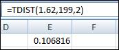
Therefore, the p-value is obtained as 0.1068.

To determine

To explain: A summary of the conclusion of the test performed above.

Expert Solution
Check Mark

Answer to Problem 71E

Solution: The two groups of early eaters and late eaters have a similar average fat consumption.

Explanation of Solution

The t-test statistic is obtained as 1.62 in the previous part. For 199 degrees of freedom, the p-value is obtained as 0.1068 using Excel. Since P>0.05, do not reject the null hypothesis and hence it is concluded that there is no significant difference between the two groups in terms of fats consumption.

(d)

To determine

To find: A 95% confidence interval for the difference of means between early eaters and late eaters in terms of consumption of fats.

(d)

Expert Solution
Check Mark

Answer to Problem 71E

Solution: The 95% confidence interval is (0.365,3.765)_.

Explanation of Solution

Calculation: The confidence interval for the difference between the means is calculated as:

Confidence interval=(x¯1x¯2)±t*s12n1+s22n2

where

x¯1=Mean of the Fat consumption by early eatersx¯2=Mean of the Fat consumption by late eaterss1=Standard deviation of Fat consumption by early eaterss2=Standard deviation of Fat consumption by late eaters

n1=Sample size of early eatersn2=Sample size of late eaterst*=t critical value for the provided confidence level

The t*–value for 95% confidence level is obtained as 1.97. Substitute the provided values in the above-defined formula to determine the 95% confidence interval as:

(x1¯x2¯)±t*s12n1+s22n2=(23.121.4)±[(1.97)×12.52202+8.22200]=1.7±[(1.97)×0.774+0.336]=1.7±2.068=(1.72.068,1.7+2.068)

=(0.368,3.768)

Therefore, the 95% confidence interval is obtained as (0.368,3.768).

To determine

To explain: The comparison of information from obtained confidence interval with the information given by the significance test.

Expert Solution
Check Mark

Answer to Problem 71E

Solution: Both the information obtained from confidence interval and the significance test shows that the null hypothesis is not rejected and concludes that there is no significant difference between the two means.

Explanation of Solution

The significance test conducted in part (c) shows that the null hypothesis is not rejected.

The obtained confidence interval (0.365,3.765) shows that the population means difference of zero lies in this interval. So, do not reject the null hypothesis H0. So, it is concluded that the information provided by both confidence interval and the significance test shows that there is no significant difference between the two means.

Want to see more full solutions like this?

Subscribe now to access step-by-step solutions to millions of textbook problems written by subject matter experts!

Chapter 7 Solutions

Introduction to the Practice of Statistics

Ch. 7.1 - Prob. 11UYKCh. 7.1 - Prob. 12UYKCh. 7.1 - Prob. 13UYKCh. 7.1 - Prob. 14ECh. 7.1 - Prob. 15ECh. 7.1 - Prob. 16ECh. 7.1 - Prob. 17ECh. 7.1 - Prob. 18ECh. 7.1 - Prob. 19ECh. 7.1 - Prob. 20ECh. 7.1 - Prob. 21ECh. 7.1 - Prob. 22ECh. 7.1 - Prob. 23ECh. 7.1 - Prob. 24ECh. 7.1 - Prob. 25ECh. 7.1 - Prob. 26ECh. 7.1 - Prob. 27ECh. 7.1 - Prob. 28ECh. 7.1 - Prob. 29ECh. 7.1 - Prob. 30ECh. 7.1 - Prob. 31ECh. 7.1 - Prob. 32ECh. 7.1 - Prob. 33ECh. 7.1 - Prob. 34ECh. 7.1 - Prob. 35ECh. 7.1 - Prob. 36ECh. 7.1 - Prob. 37ECh. 7.1 - Prob. 38ECh. 7.1 - Prob. 39ECh. 7.1 - Prob. 40ECh. 7.1 - Prob. 41ECh. 7.1 - Prob. 42ECh. 7.1 - Prob. 43ECh. 7.1 - Prob. 44ECh. 7.1 - Prob. 45ECh. 7.1 - Prob. 46ECh. 7.1 - Prob. 47ECh. 7.2 - Prob. 48UYKCh. 7.2 - Prob. 49UYKCh. 7.2 - Prob. 50UYKCh. 7.2 - Prob. 51UYKCh. 7.2 - Prob. 52UYKCh. 7.2 - Prob. 53UYKCh. 7.2 - Prob. 54UYKCh. 7.2 - Prob. 55ECh. 7.2 - Prob. 56ECh. 7.2 - Prob. 57ECh. 7.2 - Prob. 58ECh. 7.2 - Prob. 59ECh. 7.2 - Prob. 61ECh. 7.2 - Prob. 62ECh. 7.2 - Prob. 63ECh. 7.2 - Prob. 64ECh. 7.2 - Prob. 65ECh. 7.2 - Prob. 66ECh. 7.2 - Prob. 67ECh. 7.2 - Prob. 68ECh. 7.2 - Prob. 69ECh. 7.2 - Prob. 70ECh. 7.2 - Prob. 71ECh. 7.2 - Prob. 72ECh. 7.2 - Prob. 73ECh. 7.2 - Prob. 74ECh. 7.2 - Prob. 75ECh. 7.2 - Prob. 76ECh. 7.2 - Prob. 77ECh. 7.2 - Prob. 78ECh. 7.2 - Prob. 79ECh. 7.2 - Prob. 80ECh. 7.2 - Prob. 81ECh. 7.2 - Prob. 82ECh. 7.2 - Prob. 83ECh. 7.2 - Prob. 84ECh. 7.2 - Prob. 85ECh. 7.2 - Prob. 86ECh. 7.2 - Prob. 87ECh. 7.2 - Prob. 88ECh. 7.2 - Prob. 89ECh. 7.2 - Prob. 90ECh. 7.2 - Prob. 91ECh. 7.2 - Prob. 92ECh. 7.3 - Prob. 93UYKCh. 7.3 - Prob. 94UYKCh. 7.3 - Prob. 95UYKCh. 7.3 - Prob. 96UYKCh. 7.3 - Prob. 97UYKCh. 7.3 - Prob. 98UYKCh. 7.3 - Prob. 99UYKCh. 7.3 - Prob. 100UYKCh. 7.3 - Prob. 101ECh. 7.3 - Prob. 102ECh. 7.3 - Prob. 103ECh. 7.3 - Prob. 104ECh. 7.3 - Prob. 105ECh. 7.3 - Prob. 106ECh. 7.3 - Prob. 107ECh. 7.3 - Prob. 108ECh. 7.3 - Prob. 109ECh. 7.3 - Prob. 110ECh. 7.3 - Prob. 111ECh. 7.3 - Prob. 112ECh. 7.3 - Prob. 113ECh. 7.3 - Prob. 114ECh. 7.3 - Prob. 115ECh. 7.3 - Prob. 116ECh. 7.3 - Prob. 117ECh. 7.3 - Prob. 118ECh. 7 - Prob. 119ECh. 7 - Prob. 120ECh. 7 - Prob. 121ECh. 7 - Prob. 122ECh. 7 - Prob. 123ECh. 7 - Prob. 124ECh. 7 - Prob. 125ECh. 7 - Prob. 126ECh. 7 - Prob. 127ECh. 7 - Prob. 128ECh. 7 - Prob. 129ECh. 7 - Prob. 130ECh. 7 - Prob. 131ECh. 7 - Prob. 132ECh. 7 - Prob. 133ECh. 7 - Prob. 134ECh. 7 - Prob. 135ECh. 7 - Prob. 136ECh. 7 - Prob. 137ECh. 7 - Prob. 138ECh. 7 - Prob. 139ECh. 7 - Prob. 140ECh. 7 - Prob. 141ECh. 7 - Prob. 142ECh. 7 - Prob. 143ECh. 7 - Prob. 144ECh. 7 - Prob. 145ECh. 7 - Prob. 146ECh. 7 - Prob. 147ECh. 7 - Prob. 148ECh. 7 - Prob. 149E
Knowledge Booster
Background pattern image
Statistics
Learn more about
Need a deep-dive on the concept behind this application? Look no further. Learn more about this topic, statistics and related others by exploring similar questions and additional content below.
Recommended textbooks for you
Text book image
MATLAB: An Introduction with Applications
Statistics
ISBN:9781119256830
Author:Amos Gilat
Publisher:John Wiley & Sons Inc
Text book image
Probability and Statistics for Engineering and th...
Statistics
ISBN:9781305251809
Author:Jay L. Devore
Publisher:Cengage Learning
Text book image
Statistics for The Behavioral Sciences (MindTap C...
Statistics
ISBN:9781305504912
Author:Frederick J Gravetter, Larry B. Wallnau
Publisher:Cengage Learning
Text book image
Elementary Statistics: Picturing the World (7th E...
Statistics
ISBN:9780134683416
Author:Ron Larson, Betsy Farber
Publisher:PEARSON
Text book image
The Basic Practice of Statistics
Statistics
ISBN:9781319042578
Author:David S. Moore, William I. Notz, Michael A. Fligner
Publisher:W. H. Freeman
Text book image
Introduction to the Practice of Statistics
Statistics
ISBN:9781319013387
Author:David S. Moore, George P. McCabe, Bruce A. Craig
Publisher:W. H. Freeman
Use of ALGEBRA in REAL LIFE; Author: Fast and Easy Maths !;https://www.youtube.com/watch?v=9_PbWFpvkDc;License: Standard YouTube License, CC-BY
Compound Interest Formula Explained, Investment, Monthly & Continuously, Word Problems, Algebra; Author: The Organic Chemistry Tutor;https://www.youtube.com/watch?v=P182Abv3fOk;License: Standard YouTube License, CC-BY
Applications of Algebra (Digit, Age, Work, Clock, Mixture and Rate Problems); Author: EngineerProf PH;https://www.youtube.com/watch?v=Y8aJ_wYCS2g;License: Standard YouTube License, CC-BY