
Concept explainers
Videos
Section 1:
To test: The significance test to test whether there is a difference in sprint speed of Elite players from the Canadian National team and a university squad.
Section 1:
Answer to Problem 58E
Solution: There is a significant difference between the sprint speed of both types of players. The t -statistic is 2.89 which lies between
Explanation of Solution
Calculation: The hypothesis is considered as that there is no difference in sprint speed of elite players and a university squad against the alternative that there is difference in the sprint speeds of the elite players and the university squad. Hence, the hypotheses are formulated as:
The two-sample t- test statistic is defined as:
Where,
The difference of means is considered as 0 points as the null hypothesis states that there is no difference between the two sets of players. Substitute the provided values in the above-defined formula to compute the two sample t statistic. So,
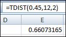
The P-value for the provided one-sided test is
So, the degree of freedom is 12. Compare the obtained value of t-statistic with the values in the table D for 12 degrees of freedom. The table D shows that the value of
To explain: The conclusion of the performed significance test.
Answer to Problem 58E
Solution: The data strongly suggests that there is a significant difference between the sprint speed of the elite players of Canadian National team and a university squad.
Explanation of Solution
Section 2:
To test: The Significance test to test whether there is difference in peak heart rate of Elite players from the Canadian National team and the university squad.
Section 2:
Answer to Problem 58E
Solution: The data strongly suggests that there is no significant difference between the peak heart rate of the elite players of Canadian National team and a university squad. The t-statistic is obtained as
Explanation of Solution
Calculation: The hypothesis is considered as that there is no difference in peak heart rate of elite players and a university squad against the alternative that there is difference in peak heart rate of the elite players and university squad. Hence, the hypotheses are formulated as:
The two-sample t- test statistic is defined as:
Where,
The difference of means is considered as 0 points as the null hypothesis states that there is no difference between the two sets of players. Substitute the provided values in the above-defined formula to compute the two sample t statistic. So,
The P-value for the provided one-sided test is
So, the degree of freedom is 12. Compare the obtained value of t- statistic with the values in the table D for 12 degrees of freedom. The table D shows that the value of
Hence, the P-value is obtained as 0.661.
To explain: The conclusion of the performed significance test.
Answer to Problem 58E
Solution: The data strongly suggests that there is no significant difference between the peak heart rate of the elite players of Canadian National team and a university squad.
Explanation of Solution
Section 3:
To test: Significance test to test whether there is difference in intermittent recovery test of Elite players from the Canadian National team and university squad.
Section 3:
Answer to Problem 58E
Solution: The data strongly suggests that there is a significant difference between the intermittent recovery test of the elite players of Canadian National team and university squad. The t- test statistic is obtained as
Explanation of Solution
Calculation: The hypothesis is considered as that there is no difference in intermittent recovery test of elite players and a university squad against the alternative that there is difference in intermittent recovery test of the elite players and university squad. Hence, the hypotheses are formulated as:
The two-sample t- test statistic is defined as:
Where
The difference of means is considered as 0 points as the null hypothesis states that there is no difference between the two sets of players. Substitute the provided values in the above-defined formula to compute the two sample t-statistic. So,
For the second approximation, the degrees of freedom k is the smaller of
So, the degree of freedom is 12. Compare the obtained value of t -statistic with the values in the table D for 12 degrees of freedom. The table D shows that the value of
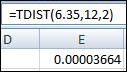
Therefore, the P-value is obtained as 0.000.
To explain: The conclusion of the performed significance test.
Answer to Problem 58E
Solution: The data strongly suggests that there is a significant difference between the intermittent recovery test of the elite players of Canadian National team and university squad.
Explanation of Solution
Want to see more full solutions like this?
Chapter 7 Solutions
Introduction to the Practice of Statistics


 MATLAB: An Introduction with ApplicationsStatisticsISBN:9781119256830Author:Amos GilatPublisher:John Wiley & Sons Inc
 Probability and Statistics for Engineering and th...StatisticsISBN:9781305251809Author:Jay L. DevorePublisher:Cengage Learning
 Statistics for The Behavioral Sciences (MindTap C...StatisticsISBN:9781305504912Author:Frederick J Gravetter, Larry B. WallnauPublisher:Cengage Learning
 Elementary Statistics: Picturing the World (7th E...StatisticsISBN:9780134683416Author:Ron Larson, Betsy FarberPublisher:PEARSON
 The Basic Practice of StatisticsStatisticsISBN:9781319042578Author:David S. Moore, William I. Notz, Michael A. FlignerPublisher:W. H. Freeman
 Introduction to the Practice of StatisticsStatisticsISBN:9781319013387Author:David S. Moore, George P. McCabe, Bruce A. CraigPublisher:W. H. Freeman