Introduction to the Practice of Statistics
9th Edition
ISBN: 9781319013387
Author: David S. Moore, George P. McCabe, Bruce A. Craig
Publisher: W. H. Freeman
bartleby

Videos

Question
Book Icon
Chapter 7.2, Problem 86E
To determine

To test: The comparison of means of the two samples using significance test of pooled methods.

Expert Solution
Check Mark

Answer to Problem 86E

Solution: The data strongly suggests that there is no significant difference between the means of early eaters and late eaters in terms of consumption of fat.

Explanation of Solution

Given: The data on total fats for early eaters and late eaters are provided. The summary of statistics fats consumption by the two groups are provided as:

x¯1=23.1x¯2=21.4s1=12.5s2=8.2

n1=202 n2=200

Explanation:

Calculation: The significance test is to compare the means of two groups in terms of consumption of fats. Hence, the null hypothesis is that the consumption of fats in the two groups is the same as against the alternative that the consumption of fats in the two groups is not same.

Therefore, the hypotheses are formulated as:

H0:μEarly=μLateHa:μEarlyμLate

In the above hypothesis, μEarly represents the average fat consumption of early eaters and μLate represents the average fat consumption of late eaters.

The two-sample t- test statistic for pooled methods is defined as:

t=(x¯1x¯2)(μ1μ2)sp1n1+1n2

where,

x¯1=Sample mean of the fat consumption by early eatersx¯2=Sample mean of the fat consumption by late eaterss1=Sample standard deviation of fat consumption by early eaterss2=Sample standard deviation of fat consumption by late eaters

n1=Sample size of fat consumption by early eatersn2=Sample size of fat consumption by late eatersμ1μ2=Difference of true population meanssp=The pooled sample standard deviation

First, determine the pooled sample standard deviation. The formula for pooled sample standard deviation is defined as:

sp=(n11)s12+(n21)s22n1+n22

Substitute the provided values and determine the pooled sample variance:

sp=[(2021)×(12.52)]+[(2001)×(8.22)]202+2002=44787.01400=10.58

Now, determine the t- statistic. The difference of means is assumed as 0 in the null hypothesis. Substitute the provided values in the above-defined formula to compute the two sample t-statistic. So,

t=(x¯1x¯2)(μ1μ2)sp1n1+1n2=(23.121.4)0(10.58)×1202+1200=1.71.06=1.60

The p-value for the provided two-sided test is calculated as P(T1.60). For the pooled two-sample t-statistic, the degrees of freedom are n1+n22. So, the degrees of freedom are calculated as:

Degrees of freedom=n1+n22 =202+2002=400

So, the degrees of freedom are 400.

The Excel function to determine the p- value from t-test statistic is displayed in the screenshot below:

Introduction to the Practice of Statistics, Chapter 7.2, Problem 86E

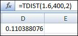
Conclusion: Therefore, the p-value is obtained as 0.1104, which is more than 0.05. So, do not reject the null hypothesis and hence it is concluded that the data strongly suggests that there is no significant difference between the means of the two groups in terms of fats consumption.

To determine

To find: A 95% confidence interval for the difference of means between early eaters and late eaters in terms of consumption of fats using pooled methods.

Expert Solution
Check Mark

Answer to Problem 86E

Solution: A 95% confidence interval is (0.3747,3.7747)_.

Explanation of Solution

Calculation: The confidence interval is calculated as:

Confidence interval=(x¯1x¯2)±t*(sp1n1+1n2)

where,

x¯1=Sample mean of the fat consumption by early eatersx¯2=Sample mean of the fat consumption by late eaterss1=Sample standard deviation of fat consumption by early eaterss2=Sample standard deviation of fat consumption by late eaters

n1=Sample size of fat consumption by early eatersn2=Sample size of fat consumption by late eatersμ1μ2=Difference of true population meanssp=The pooled sample standard deviation

The pooled sample variance is obtained as 10.58 in the previous part. The critical value of t for 95% confidence level and 400 degrees of freedom is 1.9659. Substitute the provided values in the above-defined formula to determine the 95% confidence interval for the difference between the mean consumption of fats of two groups. So,

(x¯1x¯2)±t*(sp1n1+1n2)=(23.121.4)±[(1.9659)×(10.58)×1202+1200]=(1.7±2.0747)=(1.72.0747,1.7+2.0747)=(0.3747,3.7747)

Interpretation: Therefore, the 95% confidence interval for the difference between the means is obtained as (0.3747,3.7747).

To determine

To explain: The results obtained in the provided problem with those obtained in Exercise 7.71.

Expert Solution
Check Mark

Answer to Problem 86E

Solution: The results are almost similar to those obtained in Exercise 7.71.

Explanation of Solution

The results of Exercise 7.71 are obtained as:

t=1.62pvalue=0.1081.

The results obtained in this provided problem are:

t=1.62pvalue=0.1104

Therefore, the results are almost similar.

Want to see more full solutions like this?

Subscribe now to access step-by-step solutions to millions of textbook problems written by subject matter experts!

Chapter 7 Solutions

Introduction to the Practice of Statistics

Ch. 7.1 - Prob. 11UYKCh. 7.1 - Prob. 12UYKCh. 7.1 - Prob. 13UYKCh. 7.1 - Prob. 14ECh. 7.1 - Prob. 15ECh. 7.1 - Prob. 16ECh. 7.1 - Prob. 17ECh. 7.1 - Prob. 18ECh. 7.1 - Prob. 19ECh. 7.1 - Prob. 20ECh. 7.1 - Prob. 21ECh. 7.1 - Prob. 22ECh. 7.1 - Prob. 23ECh. 7.1 - Prob. 24ECh. 7.1 - Prob. 25ECh. 7.1 - Prob. 26ECh. 7.1 - Prob. 27ECh. 7.1 - Prob. 28ECh. 7.1 - Prob. 29ECh. 7.1 - Prob. 30ECh. 7.1 - Prob. 31ECh. 7.1 - Prob. 32ECh. 7.1 - Prob. 33ECh. 7.1 - Prob. 34ECh. 7.1 - Prob. 35ECh. 7.1 - Prob. 36ECh. 7.1 - Prob. 37ECh. 7.1 - Prob. 38ECh. 7.1 - Prob. 39ECh. 7.1 - Prob. 40ECh. 7.1 - Prob. 41ECh. 7.1 - Prob. 42ECh. 7.1 - Prob. 43ECh. 7.1 - Prob. 44ECh. 7.1 - Prob. 45ECh. 7.1 - Prob. 46ECh. 7.1 - Prob. 47ECh. 7.2 - Prob. 48UYKCh. 7.2 - Prob. 49UYKCh. 7.2 - Prob. 50UYKCh. 7.2 - Prob. 51UYKCh. 7.2 - Prob. 52UYKCh. 7.2 - Prob. 53UYKCh. 7.2 - Prob. 54UYKCh. 7.2 - Prob. 55ECh. 7.2 - Prob. 56ECh. 7.2 - Prob. 57ECh. 7.2 - Prob. 58ECh. 7.2 - Prob. 59ECh. 7.2 - Prob. 61ECh. 7.2 - Prob. 62ECh. 7.2 - Prob. 63ECh. 7.2 - Prob. 64ECh. 7.2 - Prob. 65ECh. 7.2 - Prob. 66ECh. 7.2 - Prob. 67ECh. 7.2 - Prob. 68ECh. 7.2 - Prob. 69ECh. 7.2 - Prob. 70ECh. 7.2 - Prob. 71ECh. 7.2 - Prob. 72ECh. 7.2 - Prob. 73ECh. 7.2 - Prob. 74ECh. 7.2 - Prob. 75ECh. 7.2 - Prob. 76ECh. 7.2 - Prob. 77ECh. 7.2 - Prob. 78ECh. 7.2 - Prob. 79ECh. 7.2 - Prob. 80ECh. 7.2 - Prob. 81ECh. 7.2 - Prob. 82ECh. 7.2 - Prob. 83ECh. 7.2 - Prob. 84ECh. 7.2 - Prob. 85ECh. 7.2 - Prob. 86ECh. 7.2 - Prob. 87ECh. 7.2 - Prob. 88ECh. 7.2 - Prob. 89ECh. 7.2 - Prob. 90ECh. 7.2 - Prob. 91ECh. 7.2 - Prob. 92ECh. 7.3 - Prob. 93UYKCh. 7.3 - Prob. 94UYKCh. 7.3 - Prob. 95UYKCh. 7.3 - Prob. 96UYKCh. 7.3 - Prob. 97UYKCh. 7.3 - Prob. 98UYKCh. 7.3 - Prob. 99UYKCh. 7.3 - Prob. 100UYKCh. 7.3 - Prob. 101ECh. 7.3 - Prob. 102ECh. 7.3 - Prob. 103ECh. 7.3 - Prob. 104ECh. 7.3 - Prob. 105ECh. 7.3 - Prob. 106ECh. 7.3 - Prob. 107ECh. 7.3 - Prob. 108ECh. 7.3 - Prob. 109ECh. 7.3 - Prob. 110ECh. 7.3 - Prob. 111ECh. 7.3 - Prob. 112ECh. 7.3 - Prob. 113ECh. 7.3 - Prob. 114ECh. 7.3 - Prob. 115ECh. 7.3 - Prob. 116ECh. 7.3 - Prob. 117ECh. 7.3 - Prob. 118ECh. 7 - Prob. 119ECh. 7 - Prob. 120ECh. 7 - Prob. 121ECh. 7 - Prob. 122ECh. 7 - Prob. 123ECh. 7 - Prob. 124ECh. 7 - Prob. 125ECh. 7 - Prob. 126ECh. 7 - Prob. 127ECh. 7 - Prob. 128ECh. 7 - Prob. 129ECh. 7 - Prob. 130ECh. 7 - Prob. 131ECh. 7 - Prob. 132ECh. 7 - Prob. 133ECh. 7 - Prob. 134ECh. 7 - Prob. 135ECh. 7 - Prob. 136ECh. 7 - Prob. 137ECh. 7 - Prob. 138ECh. 7 - Prob. 139ECh. 7 - Prob. 140ECh. 7 - Prob. 141ECh. 7 - Prob. 142ECh. 7 - Prob. 143ECh. 7 - Prob. 144ECh. 7 - Prob. 145ECh. 7 - Prob. 146ECh. 7 - Prob. 147ECh. 7 - Prob. 148ECh. 7 - Prob. 149E
Knowledge Booster
Background pattern image
Statistics
Learn more about
Need a deep-dive on the concept behind this application? Look no further. Learn more about this topic, statistics and related others by exploring similar questions and additional content below.
Recommended textbooks for you
Text book image
MATLAB: An Introduction with Applications
Statistics
ISBN:9781119256830
Author:Amos Gilat
Publisher:John Wiley & Sons Inc
Text book image
Probability and Statistics for Engineering and th...
Statistics
ISBN:9781305251809
Author:Jay L. Devore
Publisher:Cengage Learning
Text book image
Statistics for The Behavioral Sciences (MindTap C...
Statistics
ISBN:9781305504912
Author:Frederick J Gravetter, Larry B. Wallnau
Publisher:Cengage Learning
Text book image
Elementary Statistics: Picturing the World (7th E...
Statistics
ISBN:9780134683416
Author:Ron Larson, Betsy Farber
Publisher:PEARSON
Text book image
The Basic Practice of Statistics
Statistics
ISBN:9781319042578
Author:David S. Moore, William I. Notz, Michael A. Fligner
Publisher:W. H. Freeman
Text book image
Introduction to the Practice of Statistics
Statistics
ISBN:9781319013387
Author:David S. Moore, George P. McCabe, Bruce A. Craig
Publisher:W. H. Freeman
F- Test or F- statistic (F- Test of Equality of Variance); Author: Prof. Arvind Kumar Sing;https://www.youtube.com/watch?v=PdUt7InTyc8;License: Standard Youtube License
Statistics 101: F-ratio Test for Two Equal Variances; Author: Brandon Foltz;https://www.youtube.com/watch?v=UWQO4gX7-lE;License: Standard YouTube License, CC-BY
Hypothesis Testing and Confidence Intervals (FRM Part 1 – Book 2 – Chapter 5); Author: Analystprep;https://www.youtube.com/watch?v=vth3yZIUlGQ;License: Standard YouTube License, CC-BY
Understanding the Levene's Test for Equality of Variances in SPSS; Author: Dr. Todd Grande;https://www.youtube.com/watch?v=udJr8V2P8Xo;License: Standard Youtube License