
Videos
The article “Effect of Environmental Factors on Steel Plate Corrosion Under Marine Immersion Conditions” (C. Soares, Y. Garbatov, and A. Zayed, Corrosion Engineering, Science and Technology, 2011:524–541) describes an experiment in which nine steel specimens were submerged in seawater at various temperatures, and the corrosion rates were measured. The results are presented in the following table (obtained by digitizing a graph).
| Temperature (°C) | Corrosion (mm/yr) |
| 26.6 | 1.58 |
| 26.0 | 1.45 |
| 27.4 | 1.13 |
| 21.7 | 0.96 |
| 14.9 | 0.99 |
| 11.3 | 1.05 |
| 15.0 | 0.82 |
| 8.7 | 0.68 |
| 8.2 | 0.56 |
- a. Construct a
scatterplot of corrosion (y) versus temperature (x). Verify that a linear model is appropriate. - b. Compute the least-squares line for predicting corrosion from temperature.
- c. Two steel specimens whose temperatures differ by 10°C are submerged in seawater. By how much would you predict their corrosion rates to differ?
- d. Predict the corrosion rate for steel submerged in seawater at a temperature of 20°C.
- e. Compute the fitted values.
- f. Compute the residuals. Which point has the residual with the largest magnitude?
- g. Compute the
correlation between temperature and corrosion rate. - h. Compute the regression sum of squares, the error sum of squares, and the total sum of squares.
- i. Divide the regression sum of squares by the total sum of squares. What is the relationship between this quantity and the
correlation coefficient ?
a.
Construct a scatterplot of corrosion (y) versus temperature (x) and also check whether the linear model is appropriate or not.
Answer to Problem 10E
The linear model is appropriate.
Explanation of Solution
Calculation:
The given information is that the data shows the temperature (°C) and corrosion (mm/yr) for 9 steel specimens.
Software Procedure:
Step-by-step procedure to obtain the scatterplot using the MINITAB software:
- Choose Graph > Scatter plot.
- Choose Simple, and then click OK.
- Under Y variables, select Corrosion.
- Under X variables, select Temperature.
- Click OK.
Output using the MINITAB software is given below:
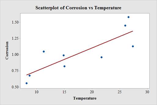
From the plot, it can be observed that the relationship between temperature and corrosion is linear. Therefore, the linear model is appropriate.
b.
Find the least-squares line for predicting corrosion from temperature.
Answer to Problem 10E
The least-squares line for predicting corrosion from temperature is
Explanation of Solution
Calculation:
Software Procedure:
Step-by-step procedure to obtain the least-squares line using the MINITAB software is given below:
- Choose Stat > Regression > Regression > Fit Regression Model.
- In Responses, enter “Corrosion”.
- In Continuous predictors, enter “Temperature”.
- Check Results.
- In Display of results, choose Simple tables.
- Click OK.
Output using the MINITAB software is given below:
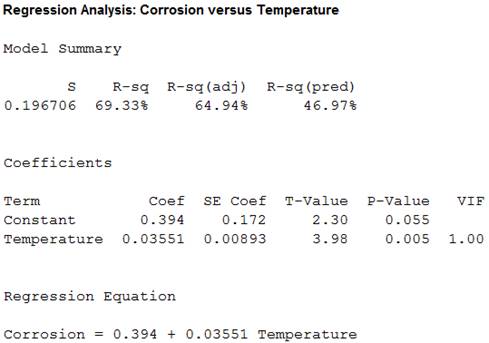
From the MINITAB output, the least-squares line for predicting corrosion from temperature is
c.
By how much would predict corrosion rates of two steel specimens to differ whose temperatures differ by 10ºC.
Explanation of Solution
Calculation:
From the least square line, the slope
The change in the predicted corrosion rates when two steel specimens whose temperatures differ by 10ºC is
Thus, the predicted corrosion rate is 0.3351 mm/yr.
d.
Predict the corrosion rate for steel submerged in seawater at a temperature of 20ºC.
Answer to Problem 10E
The predicted corrosion rate for steel submerged in seawater at a temperature of 20ºC is 1.10414 mm/yr.
Explanation of Solution
Calculation:
Predicted value:
Software Procedure:
Step-by-step procedure to obtain the predicted value using the MINITAB software:
- Stat > Regression > Regression > Predict.
- In Responses, enter “Corrosion”.
- Choose Enter individual values.
- In Temperature, enter 20.
- Click OK.
Output using the MINITAB software is given below:
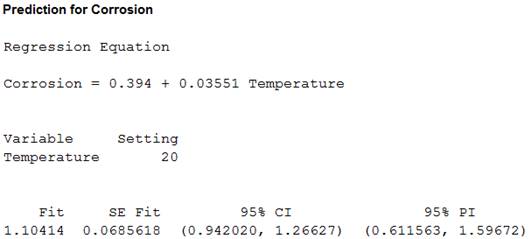
From the MINITAB output, the predicted corrosion rate for steel submerged in seawater at a temperature of 20ºC is 1.10414 mm/yr.
e.
Find the fitted values.
Answer to Problem 10E
The fitted values are, 1.33850, 1.31720, 1.36691, 1.16451, 0.92305, 0.79521, 0.92660, 0.70289 and 0.68513.
Explanation of Solution
Calculation:
Fitted value:
Software Procedure:
Step-by-step procedure to obtain the fitted value using the MINITAB software is given below:
- Choose Stat > Regression > Regression > Fit Regression Model.
- In Responses, enter “Corrosion”.
- In Continuous predictors, enter “Temperature”.
- Check Results.
- In Display of results, choose Simple tables.
- In Storage, select fits.
- Click OK.
Data display:
- Choose Data > Display data.
- In Columns, constants, and matrices to display, select FITS 1.
Output using the MINITAB software is given below:

The fitted values are, 1.33850, 1.31720, 1.36691, 1.16451, 0.92305, 0.79521, 0.92660, 0.70289 and 0.68513.
f.
Find the residuals and identify the point whose residual has the largest magnitude.
Answer to Problem 10E
The residual points are 0.241497, 0.132802, –0.236911, –0.204508, 0.066954,0.254787, –0.106597, –0.022889 and –0.125135.
The point whose residual has the largest magnitude is (11.3, 1.05).
Explanation of Solution
Calculation:
Residuals:
Software Procedure:
Step-by-step procedure to obtain the fitted value using the MINITAB software is given below:
- Choose Stat > Regression > Regression > Fit Regression Model.
- In Responses, enter “Corrosion”.
- In Continuous predictors, enter “Temperature”.
- Check Results.
- In Display of results, choose Simple tables.
- In Storage, select residuals.
- Click OK.
Data display:
- Choose Data > Display data.
- In Columns, constants, and matrices to display, select RESI 1.
Output using the MINITAB software is given below:
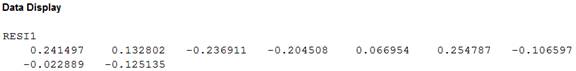
The residual points are 0.241497, 0.132802, –0.236911, –0.204508, 0.066954, 0.254787, –0.106597, –0.022889 and –0.125135.
Therefore, the point whose residual has the largest magnitude is (11.3, 1.05) because this point has the largest residual.
g.
Find the correlation between temperature and corrosion rate.
Answer to Problem 10E
The correlation between temperature and corrosion rate is 0.833.
Explanation of Solution
Calculation:
Correlation:
Software Procedure:
Step-by-step procedure to obtain the correlation using the MINITAB software:
- Select Stat > Basic Statistics > Correlation.
- In Variables, select Temperature and corrosion rate.
- Click OK.
Output using the MINITAB software is given below:
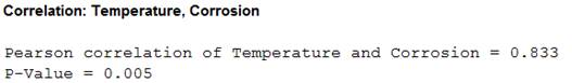
Thus, the correlation between temperature and corrosion rate is 0.833.
h.
Find the regression sum of squares, the error sum of squares, and the total sum of squares.
Answer to Problem 10E
The regression sum of squares is 0.6122, the error sum of squares is 0.2709 and the total sum of squares is 0.8830.
Explanation of Solution
Calculation:
Step-by-step procedure to obtain the regression sum of squares, the error sum of squares, and the total sum of squares using the MINITAB software is given below:
- Choose Stat > Regression > Regression > Fit Regression Model.
- In Responses, enter “Corrosion”.
- In Continuous predictors, enter “Temperature”.
- Check Results.
- In Display of results, choose Simple tables.
- Click OK.
Output using the MINITAB software is given below:
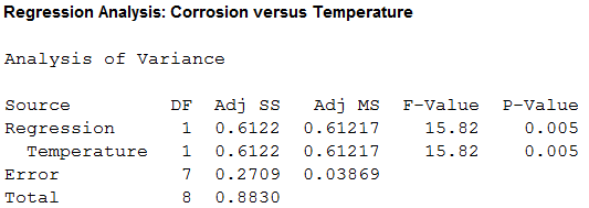
From the output, the regression sum of squares is 0.6122, the error sum of squares is 0.2709 and the total sum of squares is 0.8830.
i.
Identify the relationship between the quantity
Answer to Problem 10E
The quantity
Explanation of Solution
Calculation:
The regression sum of squares divided by the total sum of squares is
This value almost closer to the
The relationship between the quantity
Thus, the quantity
Want to see more full solutions like this?
Chapter 7 Solutions
Statistics for Engineers and Scientists
Additional Math Textbook Solutions
Business Analytics
Elementary Statistics: A Step By Step Approach
Introduction to Statistical Quality Control
Statistics for Psychology
Developmental Mathematics (9th Edition)


- An article reported data from a study in which both a baseline gasoline mixture and a reformulated gasoline were used. Consider the following observations on age (yr) and NOx emissions (g/kWh): Engine 1 2 3 4 5 6 7 8 9 10 Age 0 0 2 11 7 16 9 0 12 4 Baseline 1.74 4.38 4.04 1.23 5.30 0.58 3.35 3.44 0.73 1.23 Reformulated 1.85 5.93 5.52 2.67 6.54 0.76 4.94 4.87 0.69 1.39 Construct scatter plots of the baseline NOx emissions versus age. Construct scatter plots of the reformulated NOx emissions versus age. What appears to be the nature of the relationship between these two variables? As age increases, emissions also increase.As age increases, emissions decrease. There is no compelling relationship between the data.arrow_forward7 How many degrees of freedom (df) are associated with two different samples, 15 participants in each sample for a study investigating the effects of illumination of productivity under two treatment conditions?arrow_forwardAn article reported data from a study in which both a baseline gasoline mixture and a reformulated gasoline were used. Consider the following observations on age (yr) and NOx emissions (g/kWh): Engine 1 2 3 4 5 6 7 8 9 10 Age 0 0 2 11 7 16 9 0 12 4 Baseline 1.70 4.38 4.06 1.24 5.29 0.59 3.35 3.45 0.73 1.22 Reformulated 1.86 5.91 5.51 2.70 6.50 0.71 4.95 4.86 0.72 1.41 Construct scatter plots of the baseline NOx emissions versus age. What appears to be the nature of the relationship between these two variables? There is no compelling relationship between the data. As age increases, emissions also increase. As age increases, emissions decrease.arrow_forward
- Consider a cohort study to compare the mortality rate of myocardial infarction (MI) in men with sedentary work (exposed group) to men with physically active work (unexposed). If in the exposed, there were 36,000 person (man) years of observation and 126 deaths whereas the unexposed had 24,000 man-years of observation and 44 deaths. Compute the following a) Mortality rate in each cohort? b) What is the relative risk of dying, comparing these 2 groups? c) What is the attributable risk of sedentary work? d) What is the attributable benefit of physical activity? e) If we assume that MI is associated with the mortality in this cohort (causality), what proportion of the disease in the higher group is potentially preventable?arrow_forwardA suburban hotel derives its revenue from its hotel and restaurant operations. Theowners are interested in the relationship between the number of rooms occupied on anightly basis and the revenue per day in the restaurant. Below is a sample of 25 days(Monday through Thursday) from last year showing the restaurant income and numberof rooms occupied.arrow_forwardIn the article “Groundwater Electromagnetic Imaging in Complex Geological and Topographical Regions: A Case Study of a Tectonic Boundary in the French Alps” (S. Houtot, P. Tarits, et al., Geophysics, 2002:1048–1060), the pH was measured for several water samples in various locations near Gittaz Lake in the French Alps. The results for 11 locations on the northern side of the lake and for 6 locations on the southern side are as follows: Northern side: 8.1 8.2 8.1 8.2 8.2 7.4 7.3 7.4 8.1 8.1 7.9 Southern side: 7.8 8.2 7.9 7.9 8.1 8.1 Find a 98% confidence interval for the difference in pH between the northern and southern side.arrow_forward
- Following is the rating of marketing aggressivity (X) and sales performance (Y) of 8 sales staffs in Glovis Co in the past year: Table Attached Question: What is the hypothesis of the study?arrow_forwardThe article “Hydrogeochemical Characteristics of Groundwater in a Mid-Western CoastalAquifer System” (S. Jeen, J. Kim, et al., Geosciences Journal, 2001:339–348) presentsmeasurements of various properties of shallow groundwater in a certain aquifer system inKorea. Following are measurements of electrical conductivity (in microsiemens percentimeter) for 23 water samples.2099 528 2030 1350 1018 384 14991265 375 424 789 810 522 513488 200 215 486 257 557 260461 500Find the mean.Find the standard deviation.Find the median.Construct a dotplot.Find the 10% trimmed mean.Find the first quartile.Find the third quartile.Find the interquartile range.Construct a boxplot.Which of the points, if any, are outliers?If a histogram were constructed, would it be skewed to the left, skewed to the right, orapproximately symmetric?arrow_forwardBlood cocaine concentration (mg/L) was determinedboth for a sample of individuals who had died fromcocaine-induced excited delirium (ED) and for a sampleof those who had died from a cocaine overdose withoutexcited delirium; survival time for people in bothgroups was at most 6 hours. The accompanying datawas read from a comparative boxplot in the article“Fatal Excited Delirium Following Cocaine Use” (J.of Forensic Sciences, 1997: 25–31). ED 0 0 0 0 .1 .1 .1 .1 .2 .2 .3 .3.3 .4 .5 .7 .8 1.0 1.5 2.7 2.83.5 4.0 8.9 9.2 11.7 21.0Non-ED 0 0 0 0 0 .1 .1 .1 .1 .2 .2 .2.3 .3 .3 .4 .5 .5 .6 .8 .9 1.01.2 1.4 1.5 1.7 2.0 3.2 3.5 4.14.3 4.8 5.0 5.6 5.9 6.0 6.4 7.98.3 8.7 9.1 9.6 9.9 11.0 11.512.2 12.7 14.0 16.6 17.8 a. Determine the medians, fourths, and fourth spreadsfor the two samples.b. Are there any outliers in either sample? Any extremeoutliers?c. Construct a comparative boxplot, and use it as abasis for comparing and contrasting the ED andnon-ED samples.arrow_forward
- Suppose a researcher is interested inthe effectiveness in a new childhood exercise program implemented in a SRS of schools across a particular county. In order to test the hypothesis that the new program decreases BMI (Kg/m2), the researcher takes a SRS of children from schools where the program is employed and a SRS from schools that do not employ the program and compares the results. Assume the following table represents the SRSs of students and their BMIs. Student intervention group BMI (kg/m2) Student control group BMI (kg/m2) A 18.6 A 21.6 B 18.2 B 18.9 C 19.5 C 19.4 D 18.9 D 22.6 E 24.1 F 23.6 A) Assuming that all the necessary conditions are met (normality, independence, etc.) carry out the appropriate statistical test to determine if the new exercise program is effective. Use an alpha level of 0.05. Do not assume equal variances.B) Construct a 95% confidence interval about your estimate for the average difference in BMI between the groups.arrow_forwardThe authors of the article “Predictive Model for PittingCorrosion in Buried Oil and Gas Pipelines”(Corrosion, 2009: 332–342) provided the data on whichtheir investigation was based.a. Consider the following sample of 61 observations onmaximum pitting depth (mm) of pipeline specimensburied in clay loam soil. 0.41 0.41 0.41 0.41 0.43 0.43 0.43 0.48 0.480.58 0.79 0.79 0.81 0.81 0.81 0.91 0.94 0.941.02 1.04 1.04 1.17 1.17 1.17 1.17 1.17 1.171.17 1.19 1.19 1.27 1.40 1.40 1.59 1.59 1.601.68 1.91 1.96 1.96 1.96 2.10 2.21 2.31 2.462.49 2.57 2.74 3.10 3.18 3.30 3.58 3.58 4.154.75 5.33 7.65 7.70 8.13 10.41 13.44Construct a stem-and-leaf display in which the twolargest values are shown in a last row labeled HI.b. Refer back to (a), and create a histogram based oneight classes with 0 as the lower limit of the firstclass and class widths of .5, .5, .5, .5, 1, 2, 5, and 5,respectively.c. The accompanying comparative boxplot fromMinitab shows plots of pitting depth for four differenttypes of soils.…arrow_forwardThe accompanying frequency distribution on depositedenergy (mJ) was extracted from the article “ExperimentalAnalysis of Laser-Induced Spark Ignition of LeanTurbulent Premixed Flames” (Combustion and Flame,2013: 1414–1427).1.0− , 2.0 5 2.0− , 2.4 112.4− , 2.6 13 2.6− , 2.8 302.8− , 3.0 46 3.0− , 3.2 663.2− , 3.4 133 3.4− , 3.6 1413.6− , 3.8 126 3.8− , 4.0 924.0− , 4.2 73 4.2− , 4.4 384.4− , 4.6 19 4.6− , 5.0 11a. What proportion of these ignition trials resulted in adeposited energy of less than 3 mJ?b. What proportion of these ignition trials resulted in adeposited energy of at least 4 mJ?c. Roughly what proportion of the trials resulted in adeposited energy of at least 3.5 mJ?d. Construct a histogram and comment on its shape.arrow_forward
 MATLAB: An Introduction with ApplicationsStatisticsISBN:9781119256830Author:Amos GilatPublisher:John Wiley & Sons Inc
 Probability and Statistics for Engineering and th...StatisticsISBN:9781305251809Author:Jay L. DevorePublisher:Cengage Learning
 Statistics for The Behavioral Sciences (MindTap C...StatisticsISBN:9781305504912Author:Frederick J Gravetter, Larry B. WallnauPublisher:Cengage Learning
 Elementary Statistics: Picturing the World (7th E...StatisticsISBN:9780134683416Author:Ron Larson, Betsy FarberPublisher:PEARSON
 The Basic Practice of StatisticsStatisticsISBN:9781319042578Author:David S. Moore, William I. Notz, Michael A. FlignerPublisher:W. H. Freeman
 Introduction to the Practice of StatisticsStatisticsISBN:9781319013387Author:David S. Moore, George P. McCabe, Bruce A. CraigPublisher:W. H. Freeman