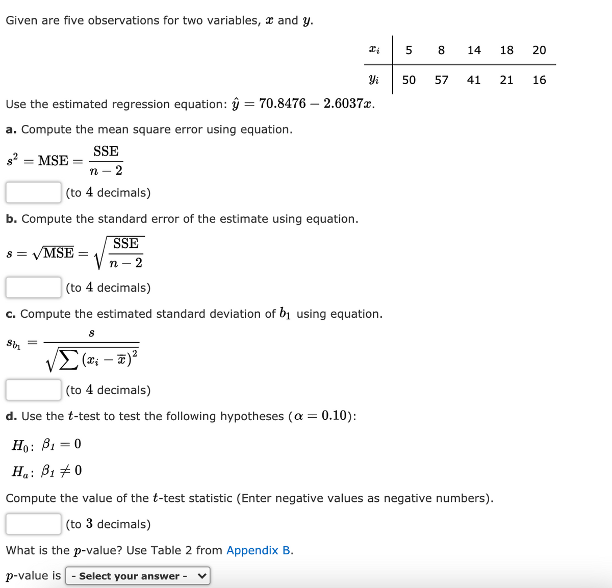
Given are five observations for two variables, x and y. 5 8 14 18 20 Yi 50 57 41 21 16 Use the estimated regression equation: ŷ = 70.8476 – 2.6037x. %3D a. Compute the mean square error using equation. SSE = MSE %3D п — 2 (to 4 decimals) b. Compute the standard error of the estimate using equation. SSE s = MSE n – 2 (to 4 decimals) c. Compute the estimated standard deviation of bị using equation. (to 4 decimals) d. Use the t-test to test the following hypotheses (a = 0.10): Ho: B1 = 0 Ha: B1 +0 Compute the value of the t-test statistic (Enter negative values as negative numbers). (to 3 decimals) What is the p-value? Use Table 2 from Appendix B. p-value is - Select your answer -


Family of Curves
A family of curves is a group of curves that are each described by a parametrization in which one or more variables are parameters. In general, the parameters have more complexity on the assembly of the curve than an ordinary linear transformation. These families appear commonly in the solution of differential equations. When a constant of integration is added, it is normally modified algebraically until it no longer replicates a plain linear transformation. The order of a differential equation depends on how many uncertain variables appear in the corresponding curve. The order of the differential equation acquired is two if two unknown variables exist in an equation belonging to this family.
XZ Plane
In order to understand XZ plane, it's helpful to understand two-dimensional and three-dimensional spaces. To plot a point on a plane, two numbers are needed, and these two numbers in the plane can be represented as an ordered pair (a,b) where a and b are real numbers and a is the horizontal coordinate and b is the vertical coordinate. This type of plane is called two-dimensional and it contains two perpendicular axes, the horizontal axis, and the vertical axis.
Euclidean Geometry
Geometry is the branch of mathematics that deals with flat surfaces like lines, angles, points, two-dimensional figures, etc. In Euclidean geometry, one studies the geometrical shapes that rely on different theorems and axioms. This (pure mathematics) geometry was introduced by the Greek mathematician Euclid, and that is why it is called Euclidean geometry. Euclid explained this in his book named 'elements'. Euclid's method in Euclidean geometry involves handling a small group of innately captivate axioms and incorporating many of these other propositions. The elements written by Euclid are the fundamentals for the study of geometry from a modern mathematical perspective. Elements comprise Euclidean theories, postulates, axioms, construction, and mathematical proofs of propositions.
Lines and Angles
In a two-dimensional plane, a line is simply a figure that joins two points. Usually, lines are used for presenting objects that are straight in shape and have minimal depth or width.
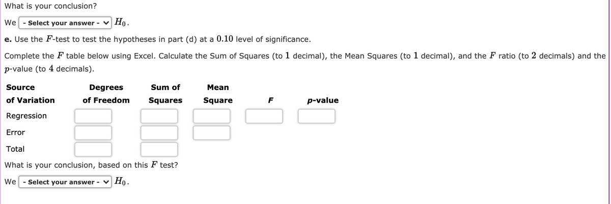
part d & e please!


Trending now
This is a popular solution!

Step by step
Solved in 4 steps with 2 images

The Wall Street Journal asked Concur Technologies, Inc., an expense management company, to examine data from million expense reports to provide insights regarding business travel expenses. Their analysis of the data showed that New York was the most expensive city. The following table shows the average daily hotel room rate () and the average amount spent on entertainment () for a random sample of of the most-visited U.S. cities. These data lead to the estimated regression equation . For these data . Click on the datafile logo to reference the data. Use Table 1 of Appendix B.
| City | Room Rate ($) |
Entertainment ($) |
| Boston | 148 | 161 |
| Denver | 96 | 105 |
| Nashville | 91 | 101 |
| New Orleans | 110 | 142 |
| Phoenix | 90 | 100 |
| San Diego | 102 | 120 |
| San Francisco | 136 | 167 |
| San Jose | 90 | 140 |
| Tampa | 82 | 98 |
a. Predict the amount spent on entertainment for a particular city that has a daily room rate of (to decimals).
b. Develop a confidence interval for the mean amount spent on entertainment for all cities that have a daily room rate of (to decimals).
to
c. The average room rate in Chicago is . Develop a prediction interval for the amount spent on entertainment in Chicago (to decimals).
to


