Mathematical Statistics with Applications
7th Edition
ISBN: 9780495110811
Author: Dennis Wackerly, William Mendenhall, Richard L. Scheaffer
Publisher: Cengage Learning
bartleby

Concept explainers

bartleby

Videos

Textbook Question
Book Icon
Chapter 11.3, Problem 6E

Applet Exercise Refer to Exercises 11.2 and 11.5. The data from Exercise 11.5 appear in the graph under the heading “Another Example” in the applet Fitting a Line Using Least Squares. Again, the horizontal blue line that initially appears on the graph is a line with 0 slope.

  1. a What is the intercept of the line with 0 slope? What is the value of SSE for the line with 0 slope?
  2. b Do you think that a line with negative slope will fit the data well? If the line is dragged to produce a negative slope, does SSE increase or decrease?
  3. c Drag the line to obtain a line that visually fits the data well. What is the equation of the line that you obtained? What is the value of SSE? What happens to SSE if the slope (and intercept) of the line is changed from the one that you visually fit?
  4. d Is the line that you visually fit the least-squares line? Click on the button “Find Best Model” to obtain the line with smallest SSE. How do the slope and intercept of the least-squares line compare to the slope and intercept of the line that you visually fit in part (c)? How do the SSEs compare?
  5. e Refer to part (a). What is the y-coordinate of the point around which the blue line pivots?
  6. f Click on the button “Display/Hide Error Squares.” What do you observe about the size of the yellow squares that appear on the graph? What is the sum of the areas of the yellow squares?

11.2 Applet Exercise How can you improve your understanding of what the method of least-squares actually does? Access the applet Fitting a Line Using Least Squares (at academic.cengage.com/statistics/wackerly). The data that appear on the first graph is from Example 11.1.

  1. a What are the slope and intercept of the blue horizontal line? (See the equation above the graph.) What is the sum of the squares of the vertical deviations between the points on the horizontal line and the observed values of the y’s? Does the horizontal line fit the data well? Click the button “Display/Hide Error Squares.” Notice that the areas of the yellow boxes are equal to the squares of the associated deviations. How does SSE compare to the sum of the areas of the yellow boxes?
  2. b Click the button “Display/Hide Error Squares” so that the yellow boxes disappear. Place the cursor on right end of the blue line. Click and hold the mouse button and drag the line so that the slope of the blue line becomes negative. What do you notice about the lengths of the vertical red lines? Did SSE increase of decrease? Does the line with negative slope appear to fit the data well?
  3. c Drag the line so that the slope is near 0.8. What happens as you move the slope closer to 0.7? Did SSE increase or decrease? When the blue line is moved, it is actually pivoting around a fixed point. What are the coordinates of that pivot point? Are the coordinates of the pivot point consistent with the result you derive in Exercise 11.1?
  4. d Drag the blue line until you obtain a line that visually fits the data well. What are the slope and intercept of the line that you visually fit to the data? What is the value of SSE for the line that you visually fit to the data? Click the button “Find Best Model” to obtain the least-squares line. How does the value of SSE compare to the SSE associated with the line that you visually fit to the data? How do the slope and intercept of the line that you visually fit to the data compare to slope and intercept of the least-squares line?

11.1 If β ^ 0 and β ^ 1 are the least-squares estimates for the intercept and slope in a simple linear regression model, show that the least-squares equation y ^ = β ^ 0 + β ^ 1 x always goes through the point ( x ¯ , y ¯ ) . [Hint: Substitute x for x in the least-squares equation and use the fact that β ^ 0 = y ¯ β ^ 1 x ¯ .]

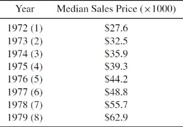
11.5 What did housing prices look like in the “good old days”? The median sale prices for new single-family houses are given in the accompanying table for the years 1972 through 1979. Letting Y denote the median sales price and x the year (using integers 1, 2, . . . , 8), fit the model Y = β0 + β1x + ε. What can you conclude from the results?

Chapter 11.3, Problem 6E, Applet Exercise Refer to Exercises 11.2 and 11.5. The data from Exercise 11.5 appear in the graph

Blurred answer

Chapter 11 Solutions

Mathematical Statistics with Applications

Ch. 11.3 - Some data obtained by C.E. Marcellari on the...Ch. 11.3 - Processors usually preserve cucumbers by...Ch. 11.3 - J. H. Matis and T. E. Wehrly report the following...Ch. 11.4 - a Derive the following identity:...Ch. 11.4 - An experiment was conducted to observe the effect...Ch. 11.4 - Prob. 17ECh. 11.4 - Prob. 18ECh. 11.4 - A study was conducted to determine the effects of...Ch. 11.4 - Suppose that Y1, Y2,,Yn are independent normal...Ch. 11.4 - Under the assumptions of Exercise 11.20, find...Ch. 11.4 - Prob. 22ECh. 11.5 - Use the properties of the least-squares estimators...Ch. 11.5 - Do the data in Exercise 11.19 present sufficient...Ch. 11.5 - Use the properties of the least-squares estimators...Ch. 11.5 - Let Y1, Y2, . . . , Yn be as given in Exercise...Ch. 11.5 - Prob. 30ECh. 11.5 - Using a chemical procedure called differential...Ch. 11.5 - Prob. 32ECh. 11.5 - Prob. 33ECh. 11.5 - Prob. 34ECh. 11.6 - For the simple linear regression model Y = 0 + 1x...Ch. 11.6 - Prob. 36ECh. 11.6 - Using the model fit to the data of Exercise 11.8,...Ch. 11.6 - Refer to Exercise 11.3. Find a 90% confidence...Ch. 11.6 - Refer to Exercise 11.16. Find a 95% confidence...Ch. 11.6 - Refer to Exercise 11.14. Find a 90% confidence...Ch. 11.6 - Prob. 41ECh. 11.7 - Suppose that the model Y=0+1+ is fit to the n data...Ch. 11.7 - Prob. 43ECh. 11.7 - Prob. 44ECh. 11.7 - Prob. 45ECh. 11.7 - Refer to Exercise 11.16. Find a 95% prediction...Ch. 11.7 - Refer to Exercise 11.14. Find a 95% prediction...Ch. 11.8 - The accompanying table gives the peak power load...Ch. 11.8 - Prob. 49ECh. 11.8 - Prob. 50ECh. 11.8 - Prob. 51ECh. 11.8 - Prob. 52ECh. 11.8 - Prob. 54ECh. 11.8 - Prob. 55ECh. 11.8 - Prob. 57ECh. 11.8 - Prob. 58ECh. 11.8 - Prob. 59ECh. 11.8 - Prob. 60ECh. 11.9 - Refer to Example 11.10. Find a 90% prediction...Ch. 11.9 - Prob. 62ECh. 11.9 - Prob. 63ECh. 11.9 - Prob. 64ECh. 11.9 - Prob. 65ECh. 11.10 - Refer to Exercise 11.3. Fit the model suggested...Ch. 11.10 - Prob. 67ECh. 11.10 - Fit the quadratic model Y=0+1x+2x2+ to the data...Ch. 11.10 - The manufacturer of Lexus automobiles has steadily...Ch. 11.10 - a Calculate SSE and S2 for Exercise 11.4. Use the...Ch. 11.12 - Consider the general linear model...Ch. 11.12 - Prob. 72ECh. 11.12 - Prob. 73ECh. 11.12 - An experiment was conducted to investigate the...Ch. 11.12 - Prob. 75ECh. 11.12 - The results that follow were obtained from an...Ch. 11.13 - Prob. 77ECh. 11.13 - Prob. 78ECh. 11.13 - Prob. 79ECh. 11.14 - Prob. 80ECh. 11.14 - Prob. 81ECh. 11.14 - Prob. 82ECh. 11.14 - Prob. 83ECh. 11.14 - Prob. 84ECh. 11.14 - Prob. 85ECh. 11.14 - Prob. 86ECh. 11.14 - Prob. 87ECh. 11.14 - Prob. 88ECh. 11.14 - Refer to the three models given in Exercise 11.88....Ch. 11.14 - Prob. 90ECh. 11.14 - Prob. 91ECh. 11.14 - Prob. 92ECh. 11.14 - Prob. 93ECh. 11.14 - Prob. 94ECh. 11 - At temperatures approaching absolute zero (273C),...Ch. 11 - A study was conducted to determine whether a...Ch. 11 - Prob. 97SECh. 11 - Prob. 98SECh. 11 - Prob. 99SECh. 11 - Prob. 100SECh. 11 - Prob. 102SECh. 11 - Prob. 103SECh. 11 - An experiment was conducted to determine the...Ch. 11 - Prob. 105SECh. 11 - Prob. 106SECh. 11 - Prob. 107SE
Knowledge Booster
Background pattern image
Statistics
Learn more about
Need a deep-dive on the concept behind this application? Look no further. Learn more about this topic, statistics and related others by exploring similar questions and additional content below.
Recommended textbooks for you
Text book image
Linear Algebra: A Modern Introduction
Algebra
ISBN:9781285463247
Author:David Poole
Publisher:Cengage Learning
Text book image
College Algebra
Algebra
ISBN:9781337282291
Author:Ron Larson
Publisher:Cengage Learning
Text book image
Algebra & Trigonometry with Analytic Geometry
Algebra
ISBN:9781133382119
Author:Swokowski
Publisher:Cengage
Correlation Vs Regression: Difference Between them with definition & Comparison Chart; Author: Key Differences;https://www.youtube.com/watch?v=Ou2QGSJVd0U;License: Standard YouTube License, CC-BY
Correlation and Regression: Concepts with Illustrative examples; Author: LEARN & APPLY : Lean and Six Sigma;https://www.youtube.com/watch?v=xTpHD5WLuoA;License: Standard YouTube License, CC-BY