
Mathematical Statistics with Applications
7th Edition
ISBN: 9780495110811
Author: Dennis Wackerly, William Mendenhall, Richard L. Scheaffer
Publisher: Cengage Learning
expand_more
expand_more
format_list_bulleted
Concept explainers
Videos
Textbook Question
Chapter 11, Problem 96SE
A study was conducted to determine whether a linear relationship exists between the breaking strength y of wooden beams and the specific gravity x of the wood. Ten randomly selected beams of the same cross-sectional dimensions were stressed until they broke. The breaking strengths and the density of the wood are shown in the accompanying table for each of the ten beams.
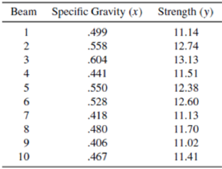
- a Fit the model Y = β0 + β1 x + ε.
- b Test H0: β1 = 0 against the alternative hypothesis, Ha: β1 ≠ 0.
- c Estimate the mean strength for beams with specific gravity .590, using a 90% confidence interval.
Expert Solution & Answer

Trending nowThis is a popular solution!

Students have asked these similar questions
The article “Mechanistic-Empirical Design of Bituminous Roads: An Indian Perspective” (A. Das and B. Pandey, Journal of Transportation Engineering, 1999:463–471) presents an equation of the form y = a(1/x1)b(1/x2)c for predicting the number of repetitions for laboratory fatigue failure (y) in terms of the tensile strain at the bottom of the bituminous beam (x1) and the resilient modulus (x2). Transform this equation into a linear model, and express the linear model coefficients in terms of a, b, and c.
Solve
An article in the ASCE Journal of Energy Engineering (1999, Vol. 125, pp.59-75) describes a study of the thermal inertia properties of autoclaved aerated concrete used as a building material. Five samples of the material were tested in a structure, and the average interior temperatures (°C) reported were as follows: 23.01, 22.22, 22.04, 22.62, and 22.59. Test that the average interior temperature is equal to 22.5°C using alpha (a) = 0.05.
1.)This problem is a test on what population parameter?
a.Variance/ Standard Deviation
b.Mean
c.Population Proportion
d.None of the above
2.)What is the null and alternative 3 points hypothesis?
a.Ho / (theta = 22.5) , Ha: (0 # 22.5)
b.Ho / (theta > 22.5) , Ha: (0 # 22.5)
c.Ho / (theta < 22.5) , Ha: (theta >= 22.5)
d.None of the above
3.)What are the Significance level 3 points and type of test?
alpha = 0.05 two-tailed
alpha = 0.95 two-tailed
alpha = 0.95 one-tailed
None of the above
4.)What standardized test statistic will…
Consider the following regression model
Yt = β0 + β1 Ut + β2 Vt + β3 Wt + β4Xt + ∈t ,
where U, V, W, X and Y are economic variables observed from t = 1, . . . , 75, β0 , . . . , β4 are the model parameters and ∈t is the random disturbance term satisfying the classical assumptions. Ordinary Least Squares (OLS) is used to estimate the parameters, producing the following estimated model:
Yt = 1.115 + 0.790*Ut − 0.327*Vt + 0.763*Wt + 0.456*Xt
(0.405) (0.178) (0.088) (0.274) (0.017)
where standard errors are given in parentheses, the R-squared = 0.941, the Durbin-Watson statistic is DW = 1.907 and the residual sum of squares is RSS = 0.0757. In answering this question, use the 5% level of significance for any hypothesis tests that you are asked to perform, state clearly the null and al- ternative hypotheses that you are testing, the test statistics that you are using and interpret the decisions that you make.…
Chapter 11 Solutions
Mathematical Statistics with Applications
Ch. 11.3 - If 0 and 1 are the least-squares estimates for the...Ch. 11.3 - Prob. 2ECh. 11.3 - Fit a straight line to the five data points in the...Ch. 11.3 - Auditors are often required to compare the audited...Ch. 11.3 - Prob. 5ECh. 11.3 - Applet Exercise Refer to Exercises 11.2 and 11.5....Ch. 11.3 - Prob. 7ECh. 11.3 - Laboratory experiments designed to measure LC50...Ch. 11.3 - Prob. 9ECh. 11.3 - Suppose that we have postulated the model...
Ch. 11.3 - Some data obtained by C.E. Marcellari on the...Ch. 11.3 - Processors usually preserve cucumbers by...Ch. 11.3 - J. H. Matis and T. E. Wehrly report the following...Ch. 11.4 - a Derive the following identity:...Ch. 11.4 - An experiment was conducted to observe the effect...Ch. 11.4 - Prob. 17ECh. 11.4 - Prob. 18ECh. 11.4 - A study was conducted to determine the effects of...Ch. 11.4 - Suppose that Y1, Y2,,Yn are independent normal...Ch. 11.4 - Under the assumptions of Exercise 11.20, find...Ch. 11.4 - Prob. 22ECh. 11.5 - Use the properties of the least-squares estimators...Ch. 11.5 - Do the data in Exercise 11.19 present sufficient...Ch. 11.5 - Use the properties of the least-squares estimators...Ch. 11.5 - Let Y1, Y2, . . . , Yn be as given in Exercise...Ch. 11.5 - Prob. 30ECh. 11.5 - Using a chemical procedure called differential...Ch. 11.5 - Prob. 32ECh. 11.5 - Prob. 33ECh. 11.5 - Prob. 34ECh. 11.6 - For the simple linear regression model Y = 0 + 1x...Ch. 11.6 - Prob. 36ECh. 11.6 - Using the model fit to the data of Exercise 11.8,...Ch. 11.6 - Refer to Exercise 11.3. Find a 90% confidence...Ch. 11.6 - Refer to Exercise 11.16. Find a 95% confidence...Ch. 11.6 - Refer to Exercise 11.14. Find a 90% confidence...Ch. 11.6 - Prob. 41ECh. 11.7 - Suppose that the model Y=0+1+ is fit to the n data...Ch. 11.7 - Prob. 43ECh. 11.7 - Prob. 44ECh. 11.7 - Prob. 45ECh. 11.7 - Refer to Exercise 11.16. Find a 95% prediction...Ch. 11.7 - Refer to Exercise 11.14. Find a 95% prediction...Ch. 11.8 - The accompanying table gives the peak power load...Ch. 11.8 - Prob. 49ECh. 11.8 - Prob. 50ECh. 11.8 - Prob. 51ECh. 11.8 - Prob. 52ECh. 11.8 - Prob. 54ECh. 11.8 - Prob. 55ECh. 11.8 - Prob. 57ECh. 11.8 - Prob. 58ECh. 11.8 - Prob. 59ECh. 11.8 - Prob. 60ECh. 11.9 - Refer to Example 11.10. Find a 90% prediction...Ch. 11.9 - Prob. 62ECh. 11.9 - Prob. 63ECh. 11.9 - Prob. 64ECh. 11.9 - Prob. 65ECh. 11.10 - Refer to Exercise 11.3. Fit the model suggested...Ch. 11.10 - Prob. 67ECh. 11.10 - Fit the quadratic model Y=0+1x+2x2+ to the data...Ch. 11.10 - The manufacturer of Lexus automobiles has steadily...Ch. 11.10 - a Calculate SSE and S2 for Exercise 11.4. Use the...Ch. 11.12 - Consider the general linear model...Ch. 11.12 - Prob. 72ECh. 11.12 - Prob. 73ECh. 11.12 - An experiment was conducted to investigate the...Ch. 11.12 - Prob. 75ECh. 11.12 - The results that follow were obtained from an...Ch. 11.13 - Prob. 77ECh. 11.13 - Prob. 78ECh. 11.13 - Prob. 79ECh. 11.14 - Prob. 80ECh. 11.14 - Prob. 81ECh. 11.14 - Prob. 82ECh. 11.14 - Prob. 83ECh. 11.14 - Prob. 84ECh. 11.14 - Prob. 85ECh. 11.14 - Prob. 86ECh. 11.14 - Prob. 87ECh. 11.14 - Prob. 88ECh. 11.14 - Refer to the three models given in Exercise 11.88....Ch. 11.14 - Prob. 90ECh. 11.14 - Prob. 91ECh. 11.14 - Prob. 92ECh. 11.14 - Prob. 93ECh. 11.14 - Prob. 94ECh. 11 - At temperatures approaching absolute zero (273C),...Ch. 11 - A study was conducted to determine whether a...Ch. 11 - Prob. 97SECh. 11 - Prob. 98SECh. 11 - Prob. 99SECh. 11 - Prob. 100SECh. 11 - Prob. 102SECh. 11 - Prob. 103SECh. 11 - An experiment was conducted to determine the...Ch. 11 - Prob. 105SECh. 11 - Prob. 106SECh. 11 - Prob. 107SE
Knowledge Booster


Learn more about
Need a deep-dive on the concept behind this application? Look no further. Learn more about this topic, statistics and related others by exploring similar questions and additional content below.Similar questions
- In a typical multiple linear regression model where x1 and x2 are non-random regressors, the expected value of the response variable y given x1 and x2 is denoted by E(y | 2,, X2). Build a multiple linear regression model for E (y | *,, *2) such that the value of E(y | x1, X2) may change as the value of x2 changes but the change in the value of E(y | X1, X2) may differ in the value of x1 . How can such a potential difference be tested and estimated statistically?arrow_forwardIn an instrumental variable regression model with one regressor, Xi, andone instrument, Zi, the regression of Xi onto Zi has R2 = 0.1 and n = 50.Is Zi a strong instrument? Would your answer change if R2 = 0.1 and n = 150?arrow_forwardin the regression specification y =α+βx +δz +ε, the parameter α is calledarrow_forward
- Consider the following two a.m. peak work trip generation models, estimated by household linear regression: T = 0.62 + 3.1 X1 + 1.4 X2 R2= 0.590 (2.3) (7.1) (5.9) T = 0.01 + 2.4 X1 + 1.2 Z1 + 4.0 Z2 R2= 0.598 (0.8) (4.2) (1.7) (3.1) X1 = number of workers in the household X2 = number of cars in the household, Z1 is a dummy variable which takes the value 1 if the household has one car, Z2 is a dummy variable which takes the value 1 if the household has two or more cars. Compare the two models and choose the best. If a zone has 1000 households, of which 50% have no car, 35% have one car, and the rest have exactly two cars, estimate the total number of trips generated by this zone. Use the preferred trip generation model and assume that each household has an average of two workersarrow_forwardThe article in the ASCE Journal of Energy Engineering (1999, Vol. 125, pp.59-75) describes a study of the thermal inertia properties of autoclaved aerated concrete used as a building material. Five samples of the material were tested in a structure, and the average interior temperatures (°C) reported were as follows: 23.01, 22.22, 22.04, 22.62, and 22.59. Test that the average interior temperature is equal to 22.5°C using alpha (a) = 0.05. This problem is a test on what population parameter? What is the null and alternative hypothesis? What are the Significance level and type of test? What standardized test statistic will be used? What is the standard test statistic? What is the Statistical Decision? What is the statistical decision in the statement form?arrow_forwardBased on the data shown below, a statistician calculates a linear model y=2.41x+2.76y=2.41x+2.76. x y 4 12.5 5 14.35 6 16.9 7 20.65 8 22.1 9 23.95 Use the model to estimate the yy-value when x=9x=9y=y=arrow_forward
- Given the following table, use the matrix method to derive the constant and slope parameters of the sample regression function: Productivity index = f(Daily sleep hours). X and Y stand for the daily sleep hours and productivity index respectively. X (Daily sleep hours) Y (Productivity index)(X first then Y in pairs so )X= 2 Y= 30 X=4 Y=35 X=5 Y=40 X=6 Y=65 X=8 Y=80arrow_forwardGiven the Z scores of: -1.5, 0.52, -1.0, 1.7 and 3.0: 1. Calculate the raw skewness and kurtosis scores for these data. 2. Calculate the standard error scores for skewness and kurtosis for these data. 3. Calculate the Z scores for skewness and kurtosis for these data.arrow_forwardThe aging Neotropical termites (Neocapritermes taracua) secrete a sticky, blue-colored liquid that they spew to intruding termites. The younger Neotropical termites secrete a liquid that lacks the blue component, so it is white in appearance. In an experiment that measured the toxicity of the blue substance, the researchers placed one drop of either the blue liquid or the white liquid on individuals of a second termite species, Labiotermes labralis. Of the 41 Labiotermes labralis that got the blue drop, 37 were immobilized. Of the 40 Labiotermes labralis that got the white drop, 9 were immobilized. Is the blue liquid toxic compared to the white liquid?arrow_forward
- f X1,X2,...,Xn constitute a random sample of size n from a geometric population, show that Y = X1 + X2 + ···+ Xn is a sufficient estimator of the parameter θ.arrow_forwardYou conduct a regression of the squared residuals against the dummy variables X1, X2, and X3 and find that for the squared residuals regression: Multiple R 0.4145 R Square 0.1718 Adjusted R Square 0.1600 SEE 92.3760 Conduct a test at the level to see if conditional heteroskedasticity is present In view of your answer for a), what needs to be done?arrow_forwardConsider the following simple linear regression model: y = β0 + β1x + u. Using a sample of n observations on x and y, you estimate the model by OLS and obtain the estimates βˆ 0, βˆ 1, and the R-squared of the regression, R2 . Then you scale this sample by a factor of 100, obtain a new sample {xi/100; yi/100} for i = 1, . . . , n, re-estimate the model by OLS, and denote the new coefficient estimates by β˜ 0, β˜ 1, and the new R-squared of the regression by R˜2 . a) Give the expression of β˜ 1 in terms of βˆ 1, and justify your answer.arrow_forward
arrow_back_ios
SEE MORE QUESTIONS
arrow_forward_ios
Recommended textbooks for you
 MATLAB: An Introduction with ApplicationsStatisticsISBN:9781119256830Author:Amos GilatPublisher:John Wiley & Sons Inc
 Probability and Statistics for Engineering and th...StatisticsISBN:9781305251809Author:Jay L. DevorePublisher:Cengage Learning
 Statistics for The Behavioral Sciences (MindTap C...StatisticsISBN:9781305504912Author:Frederick J Gravetter, Larry B. WallnauPublisher:Cengage Learning
 Elementary Statistics: Picturing the World (7th E...StatisticsISBN:9780134683416Author:Ron Larson, Betsy FarberPublisher:PEARSON
 The Basic Practice of StatisticsStatisticsISBN:9781319042578Author:David S. Moore, William I. Notz, Michael A. FlignerPublisher:W. H. Freeman
 Introduction to the Practice of StatisticsStatisticsISBN:9781319013387Author:David S. Moore, George P. McCabe, Bruce A. CraigPublisher:W. H. Freeman
MATLAB: An Introduction with Applications
Statistics
ISBN:9781119256830
Author:Amos Gilat
Publisher:John Wiley & Sons Inc
Probability and Statistics for Engineering and th...
Statistics
ISBN:9781305251809
Author:Jay L. Devore
Publisher:Cengage Learning
Statistics for The Behavioral Sciences (MindTap C...
Statistics
ISBN:9781305504912
Author:Frederick J Gravetter, Larry B. Wallnau
Publisher:Cengage Learning
Elementary Statistics: Picturing the World (7th E...
Statistics
ISBN:9780134683416
Author:Ron Larson, Betsy Farber
Publisher:PEARSON
The Basic Practice of Statistics
Statistics
ISBN:9781319042578
Author:David S. Moore, William I. Notz, Michael A. Fligner
Publisher:W. H. Freeman
Introduction to the Practice of Statistics
Statistics
ISBN:9781319013387
Author:David S. Moore, George P. McCabe, Bruce A. Craig
Publisher:W. H. Freeman
Statistics 4.1 Point Estimators; Author: Dr. Jack L. Jackson II;https://www.youtube.com/watch?v=2MrI0J8XCEE;License: Standard YouTube License, CC-BY
Statistics 101: Point Estimators; Author: Brandon Foltz;https://www.youtube.com/watch?v=4v41z3HwLaM;License: Standard YouTube License, CC-BY
Central limit theorem; Author: 365 Data Science;https://www.youtube.com/watch?v=b5xQmk9veZ4;License: Standard YouTube License, CC-BY
Point Estimate Definition & Example; Author: Prof. Essa;https://www.youtube.com/watch?v=OTVwtvQmSn0;License: Standard Youtube License
Point Estimation; Author: Vamsidhar Ambatipudi;https://www.youtube.com/watch?v=flqhlM2bZWc;License: Standard Youtube License