
Mathematical Statistics with Applications
7th Edition
ISBN: 9780495110811
Author: Dennis Wackerly, William Mendenhall, Richard L. Scheaffer
Publisher: Cengage Learning
expand_more
expand_more
format_list_bulleted
Concept explainers
Videos
Textbook Question
Chapter 11.4, Problem 16E
An experiment was conducted to observe the effect of an increase in temperature on the potency of an antibiotic. Three 1-ounce portions of the antibiotic were stored for equal lengths of time at each of the following Fahrenheit temperatures: 30◦, 50◦, 70◦, and 90◦. The potency readings observed at the end of the experimental period were as shown in the following table.
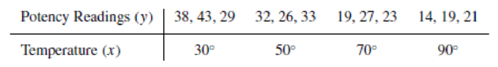
- a Find the least-squares line appropriate for this data.
- b Plot the points and graph the line as a check on your calculations.
- c Calculate S2.
Expert Solution & Answer
Want to see the full answer?
Check out a sample textbook solution
Students have asked these similar questions
Read the following description of a data set.
Charles's landscape architecture firm won a contract to design a new public
playground in Seville. To decide how many swings to include, Charles collected
information about other playgrounds in the city.
For each playground, he recorded the area (in square metres), x, and the
number of swings, y.
The least squares regression line of this data set is:
y = 0.106x + 6.784
Complete the following sentence:
For each additional square metre of area, the least squares regression line predicts that a
playground would have
more swings.
Roy's Texaco wants to keep the price of its unleaded gasoline competitive with that of other stations in the area. Roy's is currently charging $1.29 per gallon. To check that the average price for this gasoline for all stations within 12-mile radius is higher than his price, Roy randomly samples the price of unleaded gasoline at ten stations located in this area. He obtains the following data for the price per gallon (in dollars):
1.7, 1.5, 2.6, 2.2, 2.4, 2.3, 2.6, 3.0, 1.4, 2.3
Set up appropriate hypotheses and test them using a significant level of .01.
Roy ‘s Texaco wants to keep the price of its unleaded gasoline competitive with that of other stations in the area. Roy’s is currently charging $1.29 per gallon. To check that the average price for this gasoline for all stations within a 15 mile radius is higher than his price, Roy randomly samples the price of unleaded gasoline at ten stations located in this area. He obtains the following data for the price per gallon (in dollars):
1.7, 1.5, 2.6, 2.2, 2.4, 2.3, 2.6, 3.0, 1.4, 2.3
Set up the appropriate hypotheses and test them using a significance level of α= .05
Chapter 11 Solutions
Mathematical Statistics with Applications
Ch. 11.3 - If 0 and 1 are the least-squares estimates for the...Ch. 11.3 - Prob. 2ECh. 11.3 - Fit a straight line to the five data points in the...Ch. 11.3 - Auditors are often required to compare the audited...Ch. 11.3 - Prob. 5ECh. 11.3 - Applet Exercise Refer to Exercises 11.2 and 11.5....Ch. 11.3 - Prob. 7ECh. 11.3 - Laboratory experiments designed to measure LC50...Ch. 11.3 - Prob. 9ECh. 11.3 - Suppose that we have postulated the model...
Ch. 11.3 - Some data obtained by C.E. Marcellari on the...Ch. 11.3 - Processors usually preserve cucumbers by...Ch. 11.3 - J. H. Matis and T. E. Wehrly report the following...Ch. 11.4 - a Derive the following identity:...Ch. 11.4 - An experiment was conducted to observe the effect...Ch. 11.4 - Prob. 17ECh. 11.4 - Prob. 18ECh. 11.4 - A study was conducted to determine the effects of...Ch. 11.4 - Suppose that Y1, Y2,,Yn are independent normal...Ch. 11.4 - Under the assumptions of Exercise 11.20, find...Ch. 11.4 - Prob. 22ECh. 11.5 - Use the properties of the least-squares estimators...Ch. 11.5 - Do the data in Exercise 11.19 present sufficient...Ch. 11.5 - Use the properties of the least-squares estimators...Ch. 11.5 - Let Y1, Y2, . . . , Yn be as given in Exercise...Ch. 11.5 - Prob. 30ECh. 11.5 - Using a chemical procedure called differential...Ch. 11.5 - Prob. 32ECh. 11.5 - Prob. 33ECh. 11.5 - Prob. 34ECh. 11.6 - For the simple linear regression model Y = 0 + 1x...Ch. 11.6 - Prob. 36ECh. 11.6 - Using the model fit to the data of Exercise 11.8,...Ch. 11.6 - Refer to Exercise 11.3. Find a 90% confidence...Ch. 11.6 - Refer to Exercise 11.16. Find a 95% confidence...Ch. 11.6 - Refer to Exercise 11.14. Find a 90% confidence...Ch. 11.6 - Prob. 41ECh. 11.7 - Suppose that the model Y=0+1+ is fit to the n data...Ch. 11.7 - Prob. 43ECh. 11.7 - Prob. 44ECh. 11.7 - Prob. 45ECh. 11.7 - Refer to Exercise 11.16. Find a 95% prediction...Ch. 11.7 - Refer to Exercise 11.14. Find a 95% prediction...Ch. 11.8 - The accompanying table gives the peak power load...Ch. 11.8 - Prob. 49ECh. 11.8 - Prob. 50ECh. 11.8 - Prob. 51ECh. 11.8 - Prob. 52ECh. 11.8 - Prob. 54ECh. 11.8 - Prob. 55ECh. 11.8 - Prob. 57ECh. 11.8 - Prob. 58ECh. 11.8 - Prob. 59ECh. 11.8 - Prob. 60ECh. 11.9 - Refer to Example 11.10. Find a 90% prediction...Ch. 11.9 - Prob. 62ECh. 11.9 - Prob. 63ECh. 11.9 - Prob. 64ECh. 11.9 - Prob. 65ECh. 11.10 - Refer to Exercise 11.3. Fit the model suggested...Ch. 11.10 - Prob. 67ECh. 11.10 - Fit the quadratic model Y=0+1x+2x2+ to the data...Ch. 11.10 - The manufacturer of Lexus automobiles has steadily...Ch. 11.10 - a Calculate SSE and S2 for Exercise 11.4. Use the...Ch. 11.12 - Consider the general linear model...Ch. 11.12 - Prob. 72ECh. 11.12 - Prob. 73ECh. 11.12 - An experiment was conducted to investigate the...Ch. 11.12 - Prob. 75ECh. 11.12 - The results that follow were obtained from an...Ch. 11.13 - Prob. 77ECh. 11.13 - Prob. 78ECh. 11.13 - Prob. 79ECh. 11.14 - Prob. 80ECh. 11.14 - Prob. 81ECh. 11.14 - Prob. 82ECh. 11.14 - Prob. 83ECh. 11.14 - Prob. 84ECh. 11.14 - Prob. 85ECh. 11.14 - Prob. 86ECh. 11.14 - Prob. 87ECh. 11.14 - Prob. 88ECh. 11.14 - Refer to the three models given in Exercise 11.88....Ch. 11.14 - Prob. 90ECh. 11.14 - Prob. 91ECh. 11.14 - Prob. 92ECh. 11.14 - Prob. 93ECh. 11.14 - Prob. 94ECh. 11 - At temperatures approaching absolute zero (273C),...Ch. 11 - A study was conducted to determine whether a...Ch. 11 - Prob. 97SECh. 11 - Prob. 98SECh. 11 - Prob. 99SECh. 11 - Prob. 100SECh. 11 - Prob. 102SECh. 11 - Prob. 103SECh. 11 - An experiment was conducted to determine the...Ch. 11 - Prob. 105SECh. 11 - Prob. 106SECh. 11 - Prob. 107SE
Knowledge Booster


Learn more about
Need a deep-dive on the concept behind this application? Look no further. Learn more about this topic, statistics and related others by exploring similar questions and additional content below.Similar questions
- Find the equation of the regression line for the following data set. x 1 2 3 y 0 3 4arrow_forwardFind the mean hourly cost when the cell phone described above is used for 240 minutes.arrow_forwardFind the least-squares equation for the following pairs of data: x = earthquake magnitude 2.9 4.2 3.3 4.5 2.6 3.2 3.4 y = depth of earthquake (in km) 5 10 11.2 10 7.9 3.9 5.5 A. y = 2.16 + 0.221x B. y = 0.221 + 2.16x C. y = 2.16 + 0.312x D. y = 0.221 + 2.82xarrow_forward
- The following table gives the gold medal times for every other Summer Olympics for the women’s 100-meter freestyle (swimming). a.Decide which variable should be the independent variable and which should be the dependent variable. b. Draw a scatter plot of the data. c. Does it appear from inspection that there is a relationship between the variables? Why or why not? d. Calculate the least squares line. Put the equation in the form of: ŷ = a + bx. e. Find the correlation coefficient. Is the decrease in times significant? f. Find the estimated gold medal time for 1932. Find the estimated time for 1984. g. Why are the answers from part f different from the chart values? h. Does it appear that a line is the best way to fit the data? Why or why not? i. Use the least-squares line to estimate the gold medal time for the next Summer Olympics. Do you think that your answer is reasonable? Why or why not?arrow_forwardRead the following description of a data set. The owner of a bicycle store wonders if the employees who take the longest lunch breaks also make the fewest bicycle sales. One day, she notes the length of each salesperson's lunch break (in minutes), x, as well as the number of bicycles he or she sold that day, y. The least squares regression line of this data set is: ŷ = -0.297x + 10.889 Complete the following sentence: If a salesperson spends one additional minute at lunch, the least squares regression line predicts he or she will sell | fewer bicycles that day. Submit еarrow_forwardPlot the data without using a box plot. Is there an association in these data between female type and fertilizations by AA sperm?arrow_forward
- 19. You might think that increasing the resources available would elevate the number of plant spe- cies that an area could support, but the evidence suggests otherwise. The data in the accompany- ing table are from the Park Grass Experiment at Rothamsted Experimental Station in the U.K., where grassland field plots have been fertilized annually for the past 150 years (collated by Harpole and Tilman 2007). The number of plant species recorded in 10 plots is given in response to the number of different nutrient types added Plot 1 2 3 4 5 6 7 8 9 10 Number of nutrients added 0 0 0 3144 E2 3 Number of plant species 36 36 32 34 33 30 20 23 21 16arrow_forwardThe data in the table represent the number of licensed drivers in various age groups and the number of fatal accidents within the age group by gender. Complete parts (a) through (c) below. Click the icon to view the data table. ... . (a) Find the least-squares regression line for males treating the number of licensed drivers as the explanatory variable, x, and the number of fatal crashes, y, as the response variable. Repeat this procedure for females. Find the least-squares regression line for males. y=x+O Data for licensed drivers by age and gender. %3D (Round the x coefficient to three decimal places as needed. Round the constant to the nearest integer as needed.) Find the least-squares regression line for females. y = Number of Number o X+ Number of Male Fatal Number of Female Fatal (Round the x coefficient to three decimal places as needed. Round the constant to the nearest integer as needed.) Licensed Drivers Crashes Licensed Drivers Crashes (b) Interpret the slope of the…arrow_forwardA large consumer goods company has been studying the effect of advertising on total profits. As part of this study, data on advertising expenditures and total sales were collected for a five-month period and are as follows:(10, 100) (15, 200) (7, 80)(12, 120) (14, 150)The first number is advertising expenditures and the second is total sales.a. Plot the data.b. Does the plot provide evidence that advertising has a positive effect on sales?c. Compute the regression coefficients, b0 and b1arrow_forward
arrow_back_ios
arrow_forward_ios
Recommended textbooks for you
 Big Ideas Math A Bridge To Success Algebra 1: Stu...AlgebraISBN:9781680331141Author:HOUGHTON MIFFLIN HARCOURTPublisher:Houghton Mifflin Harcourt
 Linear Algebra: A Modern IntroductionAlgebraISBN:9781285463247Author:David PoolePublisher:Cengage Learning
 Glencoe Algebra 1, Student Edition, 9780079039897...AlgebraISBN:9780079039897Author:CarterPublisher:McGraw Hill
 Trigonometry (MindTap Course List)TrigonometryISBN:9781337278461Author:Ron LarsonPublisher:Cengage Learning
 Functions and Change: A Modeling Approach to Coll...AlgebraISBN:9781337111348Author:Bruce Crauder, Benny Evans, Alan NoellPublisher:Cengage Learning
Big Ideas Math A Bridge To Success Algebra 1: Stu...
Algebra
ISBN:9781680331141
Author:HOUGHTON MIFFLIN HARCOURT
Publisher:Houghton Mifflin Harcourt
Linear Algebra: A Modern Introduction
Algebra
ISBN:9781285463247
Author:David Poole
Publisher:Cengage Learning
Glencoe Algebra 1, Student Edition, 9780079039897...
Algebra
ISBN:9780079039897
Author:Carter
Publisher:McGraw Hill
Trigonometry (MindTap Course List)
Trigonometry
ISBN:9781337278461
Author:Ron Larson
Publisher:Cengage Learning
Functions and Change: A Modeling Approach to Coll...
Algebra
ISBN:9781337111348
Author:Bruce Crauder, Benny Evans, Alan Noell
Publisher:Cengage Learning
Correlation Vs Regression: Difference Between them with definition & Comparison Chart; Author: Key Differences;https://www.youtube.com/watch?v=Ou2QGSJVd0U;License: Standard YouTube License, CC-BY
Correlation and Regression: Concepts with Illustrative examples; Author: LEARN & APPLY : Lean and Six Sigma;https://www.youtube.com/watch?v=xTpHD5WLuoA;License: Standard YouTube License, CC-BY