Chapter 5, Problem 25P

(a)

To determine

Draw the time-series plot for the given data.

Identify the pattern.

Explanation of Solution

Step-by-step procedure to construct time-series plot is given below.

• Enter the data in columns A and B. Select the data.
• Click on Insert tab and then click on line.
• Select line with markers

The output is given below:

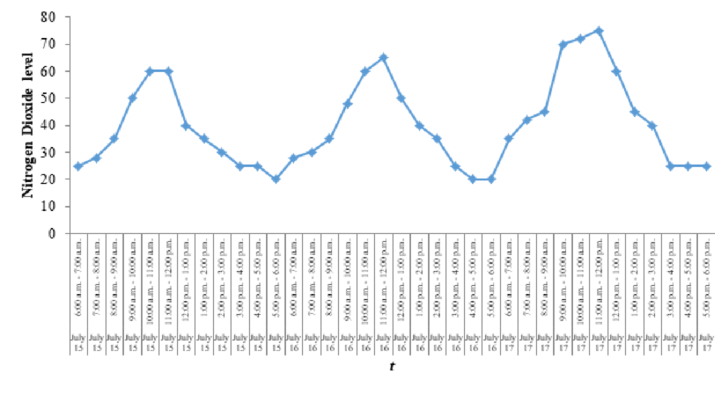
From the above time-series plot, it is clear that plot shows upward trend. Also, there exists seasonal pattern.

(b)

To determine

Find a multiple regression equation that represents seasonal effect using dummy variables for the given data.

Answer to Problem 25P

The regression equation is,

$\begin{array}{l}{\widehat{y}}_t=21.67+7.67\text{ Hour1}+11.67\text{ Hour2}+16.67\text{ Hour3}+34.33\text{ Hour4}+42.33\text{ Hour5}\\ +45\text{ Hour6}+28.33\text{ Hour7}+18.33\text{ Hour8}+13.33\text{ Hour9}+3.33\text{ Hour10}+1.67\text{ Hour11}\end{array}$.

Explanation of Solution

Dummy variables are defined as given below:

$\begin{array}{l}\text{Hour1}=\{\begin{array}{cc}1& \text{if reading was made between 6:00 a}\text{.m}\text{. and 7:00 a}\text{.m}\text{.}\\ 0& \text{otherwise}\end{array}\\ \text{Hour2}=\{\begin{array}{cc}1& \text{if reading was made between 7:00 a}\text{.m}\text{. and 8:00 a}\text{.m}\text{.}\\ 0& \text{otherwise}\end{array}\\ ⋮\\ \text{Hour11}=\{\begin{array}{cc}1& \text{if reading was made between 4:00 p}\text{.m}\text{. and 5:00 p}\text{.m}\text{.}\\ 0& \text{otherwise}\end{array}\end{array}$

Also, all the dummy variables are 0 when the reading time corresponds to 5:00 p.m. to 6:00 p.m.

The given data is entered as given below:

			Hourly Dummy Variables
Date	Hour	yt	1	2	3	4	5	6	7	8	9	10	11
July 15	6:00 a.m. - 7:00 a.m.	25	1	0	0	0	0	0	0	0	0	0	0
July 15	7:00 a.m. - 8:00 a.m.	28	0	1	0	0	0	0	0	0	0	0	0
July 15	8:00 a.m. - 9:00 a.m.	35	0	0	1	0	0	0	0	0	0	0	0
July 15	9:00 a.m. - 10:00 a.m.	50	0	0	0	1	0	0	0	0	0	0	0
July 15	10:00 a.m. - 11:00 a.m.	60	0	0	0	0	1	0	0	0	0	0	0
July 15	11:00 a.m. - 12:00 p.m.	60	0	0	0	0	0	1	0	0	0	0	0
July 15	12:00 p.m. - 1:00 p.m.	40	0	0	0	0	0	0	1	0	0	0	0
July 15	1:00 p.m. - 2:00 p.m.	35	0	0	0	0	0	0	0	1	0	0	0
July 15	2:00 p.m. - 3:00 p.m.	30	0	0	0	0	0	0	0	0	1	0	0
July 15	3:00 p.m. - 4:00 p.m.	25	0	0	0	0	0	0	0	0	0	1	0
July 15	4:00 p.m. - 5:00 p.m.	25	0	0	0	0	0	0	0	0	0	0	1
July 15	5:00 p.m. - 6:00 p.m.	20	0	0	0	0	0	0	0	0	0	0	0
July 16	6:00 a.m. - 7:00 a.m.	28	1	0	0	0	0	0	0	0	0	0	0
July 16	7:00 a.m. - 8:00 a.m.	30	0	1	0	0	0	0	0	0	0	0	0
July 16	8:00 a.m. - 9:00 a.m.	35	0	0	1	0	0	0	0	0	0	0	0
July 16	9:00 a.m. - 10:00 a.m.	48	0	0	0	1	0	0	0	0	0	0	0
July 16	10:00 a.m. - 11:00 a.m.	60	0	0	0	0	1	0	0	0	0	0	0
July 16	11:00 a.m. - 12:00 p.m.	65	0	0	0	0	0	1	0	0	0	0	0
July 16	12:00 p.m. - 1:00 p.m.	50	0	0	0	0	0	0	1	0	0	0	0
July 16	1:00 p.m. - 2:00 p.m.	40	0	0	0	0	0	0	0	1	0	0	0
July 16	2:00 p.m. - 3:00 p.m.	35	0	0	0	0	0	0	0	0	1	0	0
July 16	3:00 p.m. - 4:00 p.m.	25	0	0	0	0	0	0	0	0	0	1	0
July 16	4:00 p.m. - 5:00 p.m.	20	0	0	0	0	0	0	0	0	0	0	1
July 16	5:00 p.m. - 6:00 p.m.	20	0	0	0	0	0	0	0	0	0	0	0
July 17	6:00 a.m. - 7:00 a.m.	35	1	0	0	0	0	0	0	0	0	0	0
July 17	7:00 a.m. - 8:00 a.m.	42	0	1	0	0	0	0	0	0	0	0	0
July 17	8:00 a.m. - 9:00 a.m.	45	0	0	1	0	0	0	0	0	0	0	0
July 17	9:00 a.m. - 10:00 a.m.	70	0	0	0	1	0	0	0	0	0	0	0
July 17	10:00 a.m. - 11:00 a.m.	72	0	0	0	0	1	0	0	0	0	0	0
July 17	11:00 a.m. - 12:00 p.m.	75	0	0	0	0	0	1	0	0	0	0	0
July 17	12:00 p.m. - 1:00 p.m.	60	0	0	0	0	0	0	1	0	0	0	0
July 17	1:00 p.m. - 2:00 p.m.	45	0	0	0	0	0	0	0	1	0	0	0
July 17	2:00 p.m. - 3:00 p.m.	40	0	0	0	0	0	0	0	0	1	0	0
July 17	3:00 p.m. - 4:00 p.m.	25	0	0	0	0	0	0	0	0	0	1	0
July 17	4:00 p.m. - 5:00 p.m.	25	0	0	0	0	0	0	0	0	0	0	1
July 17	5:00 p.m. - 6:00 p.m.	25	0	0	0	0	0	0	0	0	0	0	0

Step-by-step procedure to obtain multiple linear regression line is given below.

• Enter the data in columns A to M.
• Click on Data tab and then Data Analysis.
• Select Regression and click ok.
• In Input Y Range select, $B$2:$B$37 and Input X Range select $C$2:$M$37
• Click Ok.

The output is given below:

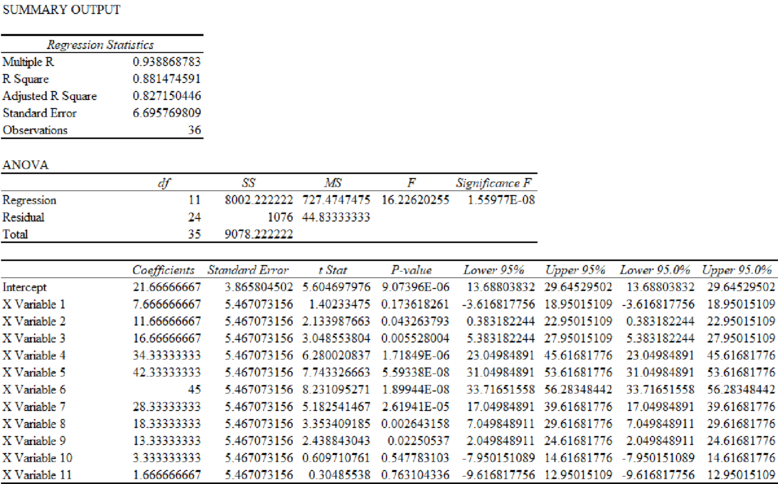
From the output the regression equation is,

$\begin{array}{l}{\widehat{y}}_t=21.67+7.67\text{ Hour1}+11.67\text{ Hour2}+16.67\text{ Hour3}+34.33\text{ Hour4}+42.33\text{ Hour5}\\ +45\text{ Hour6}+28.33\text{ Hour7}+18.33\text{ Hour8}+13.33\text{ Hour9}+3.33\text{ Hour10}+1.67\text{ Hour11}\end{array}$.

Here, X Variable 1 represents Hour1, X Variable 2 represents Hour2, … X variable 11 represents Hour11.

(c)

To determine

Find the estimates of the levels of nitrogen for July 18 using the model developed in part (b).

Explanation of Solution

From part (b), the regression equation is,

$\begin{array}{l}{\widehat{y}}_t=21.67+7.67\text{ Hour1}+11.67\text{ Hour2}+16.67\text{ Hour3}+34.33\text{ Hour4}+42.33\text{ Hour5}\\ +45\text{ Hour6}+28.33\text{ Hour7}+18.33\text{ Hour8}+13.33\text{ Hour9}+3.33\text{ Hour10}+1.67\text{ Hour11}\end{array}$

Forecast for July 18 is obtained as given below:

Hourly forecast	Calculation	${\widehat{y}}_t$
Hour1	$21.67+7.67\left(1\right)$	29.34
Hour2	$21.67+11.67\left(1\right)$	33.34
Hour3	$21.67+16.67\left(1\right)$	38.34
Hour4	$21.67+34.33\left(1\right)$	56
Hour5	$21.67+42.33\left(1\right)$	64
Hour6	$21.67+45\left(1\right)$	66.67
Hour7	$21.67+28.33\left(1\right)$	50
Hour8	$21.67+18.33\left(1\right)$	40
Hour9	$21.67+13.33\left(1\right)$	35
Hour10	$21.67+3.33\left(1\right)$	25
Hour11	$21.67+1.67\left(1\right)$	23.34
Hour12	21.67	21.67

(d)

To determine

Construct a multiple regression equation that represents seasonal effect using dummy variables and a t variable for the given data.

Answer to Problem 25P

The regression equation is,

${\widehat{y}}_t=\{\begin{array}{l}11.17+12.48\text{ Hour1}+16.04\text{ Hour2}+20.60\text{ Hour3}+37.83\text{ Hour4}+45.40\text{ Hour5}\\ +47.63\text{ Hour6}+30.52\text{ Hour7}+20.08\text{ Hour8}+14.65\text{ Hour9}+4.21\text{ Hour10}\\ +2.10\text{ Hour11}+\text{0}\text{.44}t\end{array}$.

Explanation of Solution

Create a variable t such that t = 1 for hour 1 on July 15, t = 2 for hour 2 on July 2, …, t = 36 for hour 12 on July 18.

The given data is entered as given below:

			Hourly Dummy Variables
Date	Hour	yt	1	2	3	4	5	6	7	8	9	10	11	t
July 15	6:00 a.m. - 7:00 a.m.	25	1	0	0	0	0	0	0	0	0	0	0	1
July 15	7:00 a.m. - 8:00 a.m.	28	0	1	0	0	0	0	0	0	0	0	0	2
July 15	8:00 a.m. - 9:00 a.m.	35	0	0	1	0	0	0	0	0	0	0	0	3
July 15	9:00 a.m. - 10:00 a.m.	50	0	0	0	1	0	0	0	0	0	0	0	4
July 15	10:00 a.m. - 11:00 a.m.	60	0	0	0	0	1	0	0	0	0	0	0	5
July 15	11:00 a.m. - 12:00 p.m.	60	0	0	0	0	0	1	0	0	0	0	0	6
July 15	12:00 p.m. - 1:00 p.m.	40	0	0	0	0	0	0	1	0	0	0	0	7
July 15	1:00 p.m. - 2:00 p.m.	35	0	0	0	0	0	0	0	1	0	0	0	8
July 15	2:00 p.m. - 3:00 p.m.	30	0	0	0	0	0	0	0	0	1	0	0	9
July 15	3:00 p.m. - 4:00 p.m.	25	0	0	0	0	0	0	0	0	0	1	0	10
July 15	4:00 p.m. - 5:00 p.m.	25	0	0	0	0	0	0	0	0	0	0	1	11
July 15	5:00 p.m. - 6:00 p.m.	20	0	0	0	0	0	0	0	0	0	0	0	12
July 16	6:00 a.m. - 7:00 a.m.	28	1	0	0	0	0	0	0	0	0	0	0	13
July 16	7:00 a.m. - 8:00 a.m.	30	0	1	0	0	0	0	0	0	0	0	0	14
July 16	8:00 a.m. - 9:00 a.m.	35	0	0	1	0	0	0	0	0	0	0	0	15
July 16	9:00 a.m. - 10:00 a.m.	48	0	0	0	1	0	0	0	0	0	0	0	16
July 16	10:00 a.m. - 11:00 a.m.	60	0	0	0	0	1	0	0	0	0	0	0	17
July 16	11:00 a.m. - 12:00 p.m.	65	0	0	0	0	0	1	0	0	0	0	0	18
July 16	12:00 p.m. - 1:00 p.m.	50	0	0	0	0	0	0	1	0	0	0	0	19
July 16	1:00 p.m. - 2:00 p.m.	40	0	0	0	0	0	0	0	1	0	0	0	20
July 16	2:00 p.m. - 3:00 p.m.	35	0	0	0	0	0	0	0	0	1	0	0	21
July 16	3:00 p.m. - 4:00 p.m.	25	0	0	0	0	0	0	0	0	0	1	0	22
July 16	4:00 p.m. - 5:00 p.m.	20	0	0	0	0	0	0	0	0	0	0	1	23
July 16	5:00 p.m. - 6:00 p.m.	20	0	0	0	0	0	0	0	0	0	0	0	24
July 17	6:00 a.m. - 7:00 a.m.	35	1	0	0	0	0	0	0	0	0	0	0	25
July 17	7:00 a.m. - 8:00 a.m.	42	0	1	0	0	0	0	0	0	0	0	0	26
July 17	8:00 a.m. - 9:00 a.m.	45	0	0	1	0	0	0	0	0	0	0	0	27
July 17	9:00 a.m. - 10:00 a.m.	70	0	0	0	1	0	0	0	0	0	0	0	28
July 17	10:00 a.m. - 11:00 a.m.	72	0	0	0	0	1	0	0	0	0	0	0	29
July 17	11:00 a.m. - 12:00 p.m.	75	0	0	0	0	0	1	0	0	0	0	0	30
July 17	12:00 p.m. - 1:00 p.m.	60	0	0	0	0	0	0	1	0	0	0	0	31
July 17	1:00 p.m. - 2:00 p.m.	45	0	0	0	0	0	0	0	1	0	0	0	32
July 17	2:00 p.m. - 3:00 p.m.	40	0	0	0	0	0	0	0	0	1	0	0	33
July 17	3:00 p.m. - 4:00 p.m.	25	0	0	0	0	0	0	0	0	0	1	0	34
July 17	4:00 p.m. - 5:00 p.m.	25	0	0	0	0	0	0	0	0	0	0	1	35
July 17	5:00 p.m. - 6:00 p.m.	25	0	0	0	0	0	0	0	0	0	0	0	36

Step-by-step procedure to obtain multiple linear regression line is given below.

• Enter the data in columns A to N.
• Click on Data tab and then Data Analysis.
• Select Regression and click ok.
• In Input Y Range select, $B$2:$B$37 and Input X Range select $C$2:$N$37
• Click Ok.

The output is given below:

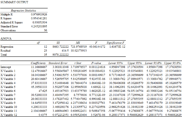
From the output the regression equation is,

${\widehat{y}}_t=\{\begin{array}{l}11.17+12.48\text{ Hour1}+16.04\text{ Hour2}+20.60\text{ Hour3}+37.83\text{ Hour4}+45.40\text{ Hour5}\\ +47.63\text{ Hour6}+30.52\text{ Hour7}+20.08\text{ Hour8}+14.65\text{ Hour9}+4.21\text{ Hour10}\\ +2.10\text{ Hour11}+\text{0}\text{.44}t\end{array}$.

Here, X Variable 1 represents Hour1, X Variable 2 represents Hour2,… X variable 11 represents Hour11 and X variable 12 represents t.

(e)

To determine

Calculate the estimates of the levels of nitrogen for July 18 using the model developed in part (d).

Explanation of Solution

From part (d), the regression equation is,

${\widehat{y}}_t=\{\begin{array}{l}11.17+12.48\text{ Hour1}+16.04\text{ Hour2}+20.60\text{ Hour3}+37.83\text{ Hour4}+45.40\text{ Hour5}\\ +47.63\text{ Hour6}+30.52\text{ Hour7}+20.08\text{ Hour8}+14.65\text{ Hour9}+4.21\text{ Hour10}\\ +2.10\text{ Hour11}+\text{0}\text{.44}t\end{array}$

Forecast for July 18 is given below:

Hourly forecast	T	Calculation	${\widehat{y}}_t$
1	37	$11.17+12.48\left(1\right)+\text{0}\text{.44}\left(37\right)$	39.93
2	38	$11.17+16.04\left(1\right)+\text{0}\text{.44}\left(38\right)$	43.93
3	39	$11.17+20.60\left(1\right)+\text{0}\text{.44}\left(39\right)$	48.93
4	40	$11.17+37.83\left(1\right)+\text{0}\text{.44}\left(40\right)$	66.6
5	41	$11.17+45.40\left(1\right)+\text{0}\text{.44}\left(41\right)$	74.71
6	42	$11.17+47.63\left(1\right)+\text{0}\text{.44}\left(42\right)$	77.28
7	43	$11.17+30.52\left(1\right)+\text{0}\text{.44}\left(43\right)$	60.61
8	44	$11.17+20.08\left(1\right)+\text{0}\text{.44}\left(44\right)$	50.61
9	45	$11.17+14.65\left(1\right)+\text{0}\text{.44}\left(45\right)$	45.62
10	46	$11.17+4.21\left(1\right)+\text{0}\text{.44}\left(46\right)$	35.62
11	47	$11.17+2.10\left(1\right)+\text{0}\text{.44}\left(47\right)$	33.95
12	48	$11.17+\text{0}\text{.44}\left(48\right)$	32.29

(f)

To determine

Justify which of the models (b) or (d) is effective.

Answer to Problem 25P

Model (d) is preferred.

Explanation of Solution

For the multiple regression equation developed in part (b), MSE is obtained as given below:

Date	Hour	yt	Forecast	Forecast Error	Squared Forecast Error
15-Jul	6:00 a.m. - 7:00 a.m.	25	29.34	-4.34	18.8356
15-Jul	7:00 a.m. - 8:00 a.m.	28	33.34	-5.34	28.5156
15-Jul	8:00 a.m. - 9:00 a.m.	35	38.34	-3.34	11.1556
15-Jul	9:00 a.m. - 10:00 a.m.	50	56	-6	36
15-Jul	10:00 a.m. - 11:00 a.m.	60	64	-4	16
15-Jul	11:00 a.m. - 12:00 p.m.	60	66.67	-6.67	44.4889
15-Jul	12:00 p.m. - 1:00 p.m.	40	50	-10	100
15-Jul	1:00 p.m. - 2:00 p.m.	35	40	-5	25
15-Jul	2:00 p.m. - 3:00 p.m.	30	35	-5	25
15-Jul	3:00 p.m. - 4:00 p.m.	25	25	0	0
15-Jul	4:00 p.m. - 5:00 p.m.	25	23.34	1.66	2.7556
15-Jul	5:00 p.m. - 6:00 p.m.	20	21.67	-1.67	2.7889
16-Jul	6:00 a.m. - 7:00 a.m.	28	29.34	-1.34	1.7956
16-Jul	7:00 a.m. - 8:00 a.m.	30	33.34	-3.34	11.1556
16-Jul	8:00 a.m. - 9:00 a.m.	35	38.34	-3.34	11.1556
16-Jul	9:00 a.m. - 10:00 a.m.	48	56	-8	64
16-Jul	10:00 a.m. - 11:00 a.m.	60	64	-4	16
16-Jul	11:00 a.m. - 12:00 p.m.	65	66.67	-1.67	2.7889
16-Jul	12:00 p.m. - 1:00 p.m.	50	50	0	0
16-Jul	1:00 p.m. - 2:00 p.m.	40	40	0	0
16-Jul	2:00 p.m. - 3:00 p.m.	35	35	0	0
16-Jul	3:00 p.m. - 4:00 p.m.	25	25	0	0
16-Jul	4:00 p.m. - 5:00 p.m.	20	23.34	-3.34	11.1556
16-Jul	5:00 p.m. - 6:00 p.m.	20	21.67	-1.67	2.7889
17-Jul	6:00 a.m. - 7:00 a.m.	35	29.34	5.66	32.0356
17-Jul	7:00 a.m. - 8:00 a.m.	42	33.34	8.66	74.9956
17-Jul	8:00 a.m. - 9:00 a.m.	45	38.34	6.66	44.3556
17-Jul	9:00 a.m. - 10:00 a.m.	70	56	14	196
17-Jul	10:00 a.m. - 11:00 a.m.	72	64	8	64
17-Jul	11:00 a.m. - 12:00 p.m.	75	66.67	8.33	69.3889
17-Jul	12:00 p.m. - 1:00 p.m.	60	50	10	100
17-Jul	1:00 p.m. - 2:00 p.m.	45	40	5	25
17-Jul	2:00 p.m. - 3:00 p.m.	40	35	5	25
17-Jul	3:00 p.m. - 4:00 p.m.	25	25	0	0
17-Jul	4:00 p.m. - 5:00 p.m.	25	23.34	1.66	2.7556
17-Jul	5:00 p.m. - 6:00 p.m.	25	21.67	3.33	11.0889
					1076.001

$\begin{array}{c}MSE=\frac{{\displaystyle {\sum }_{}^{}{\left|e_r\right|}^2}}{n-k}\\ =\frac{1076.001}{36}\\ =29.89\end{array}$

For the multiple regression equation developed in part (d), MSE is obtained as given below:

Date	Hour	t	yt	Forecast	Forecast Error	Squared Forecast Error
15-Jul	6:00 a.m. - 7:00 a.m.	1	25	24.09	0.91	0.8281
15-Jul	7:00 a.m. - 8:00 a.m.	2	28	28.09	-0.09	0.0081
15-Jul	8:00 a.m. - 9:00 a.m.	3	35	33.09	1.91	3.6481
15-Jul	9:00 a.m. - 10:00 a.m.	4	50	50.76	-0.76	0.5776
15-Jul	10:00 a.m. - 11:00 a.m.	5	60	58.87	1.13	1.2769
15-Jul	11:00 a.m. - 12:00 p.m.	6	60	61.44	-1.44	2.0736
15-Jul	12:00 p.m. - 1:00 p.m.	7	40	44.77	-4.77	22.7529
15-Jul	1:00 p.m. - 2:00 p.m.	8	35	34.77	0.23	0.0529
15-Jul	2:00 p.m. - 3:00 p.m.	9	30	29.78	0.22	0.0484
15-Jul	3:00 p.m. - 4:00 p.m.	10	25	19.78	5.22	27.2484
15-Jul	4:00 p.m. - 5:00 p.m.	11	25	18.11	6.89	47.4721
15-Jul	5:00 p.m. - 6:00 p.m.	12	20	16.45	3.55	12.6025
16-Jul	6:00 a.m. - 7:00 a.m.	13	28	29.37	-1.37	1.8769
16-Jul	7:00 a.m. - 8:00 a.m.	14	30	33.37	-3.37	11.3569
16-Jul	8:00 a.m. - 9:00 a.m.	15	35	38.37	-3.37	11.3569
16-Jul	9:00 a.m. - 10:00 a.m.	16	48	56.04	-8.04	64.6416
16-Jul	10:00 a.m. - 11:00 a.m.	17	60	64.15	-4.15	17.2225
16-Jul	11:00 a.m. - 12:00 p.m.	18	65	66.72	-1.72	2.9584
16-Jul	12:00 p.m. - 1:00 p.m.	19	50	50.05	-0.05	0.0025
16-Jul	1:00 p.m. - 2:00 p.m.	20	40	40.05	-0.05	0.0025
16-Jul	2:00 p.m. - 3:00 p.m.	21	35	35.06	-0.06	0.0036
16-Jul	3:00 p.m. - 4:00 p.m.	22	25	25.06	-0.06	0.0036
16-Jul	4:00 p.m. - 5:00 p.m.	23	20	23.39	-3.39	11.4921
16-Jul	5:00 p.m. - 6:00 p.m.	24	20	21.73	-1.73	2.9929
17-Jul	6:00 a.m. - 7:00 a.m.	25	35	34.65	0.35	0.1225
17-Jul	7:00 a.m. - 8:00 a.m.	26	42	38.65	3.35	11.2225
17-Jul	8:00 a.m. - 9:00 a.m.	27	45	43.65	1.35	1.8225
17-Jul	9:00 a.m. - 10:00 a.m.	28	70	61.32	8.68	75.3424
17-Jul	10:00 a.m. - 11:00 a.m.	29	72	69.43	2.57	6.6049
17-Jul	11:00 a.m. - 12:00 p.m.	30	75	72	3	9
17-Jul	12:00 p.m. - 1:00 p.m.	31	60	55.33	4.67	21.8089
17-Jul	1:00 p.m. - 2:00 p.m.	32	45	45.33	-0.33	0.1089
17-Jul	2:00 p.m. - 3:00 p.m.	33	40	40.34	-0.34	0.1156
17-Jul	3:00 p.m. - 4:00 p.m.	34	25	30.34	-5.34	28.5156
17-Jul	4:00 p.m. - 5:00 p.m.	35	25	28.67	-3.67	13.4689
17-Jul	5:00 p.m. - 6:00 p.m.	36	25	27.01	-2.01	4.0401
						414.6728

$\begin{array}{c}MSE=\frac{{\displaystyle {\sum }_{}^{}{\left|e_r\right|}^2}}{n-k}\\ =\frac{414.6728}{36}\\ =11.52\end{array}$

MSE for model in (d) is smaller than MSE for the model in (b). Thus, model (d) is preferred.