Essentials Of Business Analytics
1st Edition
ISBN: 9781285187273
Author: Camm, Jeff.
Publisher: Cengage Learning,
expand_more
expand_more
format_list_bulleted
Concept explainers
Videos
Textbook Question
Chapter 5, Problem 26P
South Shore Construction builds permanent docks and seawalls along the southern shore of Long Island, New York. Although the firm has been in business only five years, revenue has increased from $308,000 in the first year of operation to $1,084,000 in the most recent year. The following data show the quarterly sales revenue in thousands of dollars:
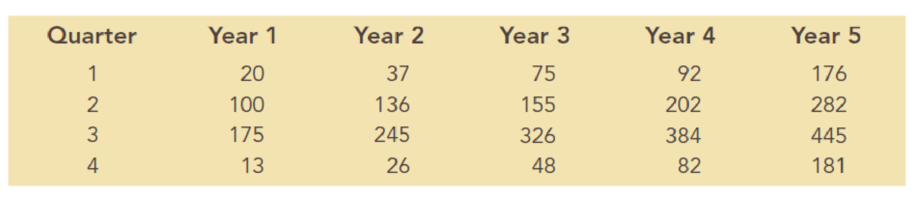
- a. Construct a time series plot. What type of pattern exists in the data?
- b. Use a multiple regression model with dummy variables as follows to develop an equation to account for seasonal effects in the data: Qtr1 = 1 if quarter I, 0 otherwise; Qtr2 = 1 if quarter 2, 0 otherwise; Qtr3 = 1 if quarter 3, 0 otherwise.
- c. Based on the model you developed in part (b), compute estimates of quarterly sales for year 6.
- d. Let Period = 1 refer to the observation in quarter 1 of year 1; Period = 2 refer to the observation in quarter 2 of year 1; … and Period = 20 refer to the observation in quarter 4 of year 5. Using the dummy variables defined in part (b) and the variable Period, develop an equation to account for seasonal effects and any linear trend in the time series.
- e. Based on the seasonal effects in the data and linear trend estimated in part (c), compute estimates of quarterly sales for year 6.
- f. Is the model you developed in part (b) or the model you developed in part (d) more effective? Justify your answer.
Expert Solution & Answer
Want to see the full answer?
Check out a sample textbook solution
Students have asked these similar questions
In the following table, the heights and salaries of the knights of 12 kingdoms have been collected. In the table, the lengths are in centimeters and the wages are in the monetary unit of the kingdom in question.
(This is the table)
Lenght Salary183 100160 92196 106186 92195 109182 101208 116169 96166 94198 101145 93168 96
So the questions regarding this table would be: (a) Fit a linear regression model to the data and determine its PNS estimates αˆ and βˆ.(b) Calculate the prediction for a knight's salary when that knight is 181 centimeters tall.(c) Estimate the variance parameter σ2 of the linear model.
R software or other software for linear regressions should not be used to solve this.
Consider the following time series:
Quarter
Year 1
Year 2
Year 3
1
66
63
57
2
48
40
50
3
59
61
54
4
73
76
67
(a)
Choose a time series plot.
(i)
(ii)
(iii)
(iv)
What type of pattern exists in the data? Is there an indication of a seasonal pattern?
(b)
Use a multiple linear regression model with dummy variables as follows to develop an equation to account for seasonal effects in the data: Qtr1 = 1 if quarter 1, 0 otherwise; Qtr2 = 1 if quarter 2, 0 otherwise; Qtr3 = 1 if quarter 3, 0 otherwise. For subtractive or negative numbers use a minus sign even if there is a + sign before the blank (Example: -300).
ŷ = ?? + ?? Qtr1 +?? Qtr2 + ?? Qtr3
(c)
Compute the quarterly forecasts for next year.
Year
Quarter
Ft
4
1
4
2
4
3
4
4
The president of small manufacturing firm is concerned about the continual increase in manufacturing costs over the past several years. The following figures provide a time series of the cost per unit for the firm’s leading product over the past eight years.
Year
Cost/Unit ($)
Year
Cost/Unit ($)
1
20.00
5
26.60
2
24.50
6
30.00
3
28.20
7
31.00
4
27.50
8
36.00
Construct a time series plot. What type of pattern exists in the data?
Use simple linear regression analysis to find the parameters for the line that minimizes MSE for this time series.
What is the average cost increase that the firm has been realizing per year?
Compute an estimate of the cost/unit for next year.
Chapter 5 Solutions
Essentials Of Business Analytics
Ch. 5 - Consider the following time series data:
Using...Ch. 5 - Refer to the time series data in Problem 1. Using...Ch. 5 - Problems 1 and 2 used different forecasting...Ch. 5 - Consider the following time series data:
Compute...Ch. 5 - Consider the following time series...Ch. 5 - Consider the following time series...Ch. 5 - Prob. 8PCh. 5 - Prob. 9PCh. 5 - Prob. 10PCh. 5 - For the Hawkins Company, the monthly percentages...
Ch. 5 - Corporate triple A bond interest rates for 12...Ch. 5 - The values of Alabama building contracts (in...Ch. 5 - The following time series shows the sales of a...Ch. 5 - Prob. 15PCh. 5 - The following table reports the percentage of...Ch. 5 - Consider the following time series: a. Construct a...Ch. 5 - Consider the following time series:
Construct a...Ch. 5 - The Seneca Children’s Fund (SCF) is a local...Ch. 5 - The president of a small manufacturing firm is...Ch. 5 - Consider the following time series: a. Construct a...Ch. 5 - Consider the following time series...Ch. 5 - The quarterly sales data (number of copies sold)...Ch. 5 - Prob. 25PCh. 5 - South Shore Construction builds permanent docks...Ch. 5 - Hogs & Dawgs is an ice cream parlor on the border...Ch. 5 - Donna Nickles manages a gasoline station on the...Ch. 5 - The Vintage Restaurant, on Captiva Island near...
Knowledge Booster


Learn more about
Need a deep-dive on the concept behind this application? Look no further. Learn more about this topic, statistics and related others by exploring similar questions and additional content below.Similar questions
- Cable TV The following table shows the number C. in millions, of basic subscribers to cable TV in the indicated year These data are from the Statistical Abstract of the United States. Year 1975 1980 1985 1990 1995 2000 C 9.8 17.5 35.4 50.5 60.6 60.6 a. Use regression to find a logistic model for these data. b. By what annual percentage would you expect the number of cable subscribers to grow in the absence of limiting factors? c. The estimated number of subscribers in 2005 was 65.3million. What light does this shed on the model you found in part a?arrow_forwardUrban Travel Times Population of cities and driving times are related, as shown in the accompanying table, which shows the 1960 population N, in thousands, for several cities, together with the average time T, in minutes, sent by residents driving to work. City Population N Driving time T Los Angeles 6489 16.8 Pittsburgh 1804 12.6 Washington 1808 14.3 Hutchinson 38 6.1 Nashville 347 10.8 Tallahassee 48 7.3 An analysis of these data, along with data from 17 other cities in the United States and Canada, led to a power model of average driving time as a function of population. a Construct a power model of driving time in minutes as a function of population measured in thousands b Is average driving time in Pittsburgh more or less than would be expected from its population? c If you wish to move to a smaller city to reduce your average driving time to work by 25, how much smaller should the city be?arrow_forward1. The following data set contains information on years of formal education and incomes in 2015. Please answer questions d-h. Questions a-c were already answered. Row Education Income in in Years 2015 Dollars 1 7 22587 2 10 28305 3 12 40196 4 13 49483 5 14 54483 6 16 78073 7 18 99540 8 19 155646 9 21 125310 a. Estimate the regression equation Income = a + b(Education). b. What is the predicted increase in Income for a one-year increase in Education? c. What do you predict Income to be for a person who has 17 years of education? d. What fraction of the variation in Income is explained (or accounted for) by Education? e. Why do you think Income (in the data set) for 21 years of Education is lower than income with 19 years of education? f. Show the graph of the data with the equation for your regression line. g. Use the F statistic to test the hypothesis that there is no relation between Income and Education at the 5% level of significance. Do you reject this hypothesis…arrow_forward
Recommended textbooks for you
 Functions and Change: A Modeling Approach to Coll...AlgebraISBN:9781337111348Author:Bruce Crauder, Benny Evans, Alan NoellPublisher:Cengage Learning
Functions and Change: A Modeling Approach to Coll...
Algebra
ISBN:9781337111348
Author:Bruce Crauder, Benny Evans, Alan Noell
Publisher:Cengage Learning
Correlation Vs Regression: Difference Between them with definition & Comparison Chart; Author: Key Differences;https://www.youtube.com/watch?v=Ou2QGSJVd0U;License: Standard YouTube License, CC-BY
Correlation and Regression: Concepts with Illustrative examples; Author: LEARN & APPLY : Lean and Six Sigma;https://www.youtube.com/watch?v=xTpHD5WLuoA;License: Standard YouTube License, CC-BY