Connect Access Card for Statistics for Engineers and Scientists
4th Edition
ISBN: 9780073518237
Author: William Navidi
Publisher: McGraw-Hill Education
expand_more
expand_more
format_list_bulleted
Concept explainers
Videos
Textbook Question
Chapter 8.1, Problem 16E
The following data were collected in an experiment to study the relationship between extrusion pressure (in KPa) and wear (in mg).
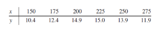
The least-squares quadratic model is y = –32.445714 + 0.43154286x – 0.000982857x2.
- a. Using this equation, compute the residuals.
- b. Compute the error sum of squares SSE and the total sum of squares SST.
- c. Compute the error variance estimate s2.
- d. Compute the coefficient of determination R2.
- e. Compute the value of the F statistic for the hypothesis H0 = β1 = β2 = 0. How many degrees of freedom does this statistic have?
- f. Can the hypothesis H0 = β1 = β2 = 0 be rejected at the 5% level? Explain.
Expert Solution & Answer
Want to see the full answer?
Check out a sample textbook solution
Students have asked these similar questions
The following Minitab display gives information regarding the relationship between the body weight of a child (in kilograms) and the metabolic rate of the child (in 100 kcal/ 24 hr).
Predictor Coef SE Coef T PConstant 0.8570 0.4148 2.06 0.84Weight 0.38243 0.02978 13.52 0.000
S = 0.517508 R-Sq = 97.4%
(a) Write out the least-squares equation.
y^= ______ + _____x
(b) For each 1 kilogram increase in weight, how much does the metabolic rate of a child increase? (Use 5 decimal places.)
The following Minitab display gives information regarding the relationship between the body weight of a child (in kilograms) and the metabolic rate of the child (in 100 kcal/ 24 hr).
Predictor
Coef
SE Coef
T
P
Constant
0.8651
0.4148
2.06
0.84
Weight
0.40619
0.02978
13.52
0.000
S = 0.517508
R-Sq = 97.0%
(a) Write out the least-squares equation.
y =
+ x
(b) For each 1 kilogram increase in weight, how much does the metabolic rate of a child increase? (Use 5 decimal places.)(c) What is the value of the correlation coefficient r? (Use 3 decimal places.)
The following information relates to BCD Co. Month Usage Cost Jan. 600 P750 Feb. 650 775 Mar. 420 550 Apr. 500 650 May 450 570Using the least squares regression, what is the fixed cost element (to the nearest whole peso)?
Chapter 8 Solutions
Connect Access Card for Statistics for Engineers and Scientists
Ch. 8.1 - In an experiment to determine the factors...Ch. 8.1 - Prob. 2ECh. 8.1 - Prob. 3ECh. 8.1 - The article Application of Analysis of Variance to...Ch. 8.1 - Prob. 5ECh. 8.1 - Prob. 6ECh. 8.1 - Prob. 7ECh. 8.1 - Refer to Exercise 7. a. Find a 95% confidence...Ch. 8.1 - In a study of the lung function of children, the...Ch. 8.1 - Prob. 10E
Ch. 8.1 - Prob. 11ECh. 8.1 - The following MINITAB output is for a multiple...Ch. 8.1 - Prob. 13ECh. 8.1 - Prob. 14ECh. 8.1 - Prob. 15ECh. 8.1 - The following data were collected in an experiment...Ch. 8.1 - The November 24, 2001, issue of The Economist...Ch. 8.1 - The article Multiple Linear Regression for Lake...Ch. 8.1 - Prob. 19ECh. 8.2 - In an experiment to determine factors related to...Ch. 8.2 - In a laboratory test of a new engine design, the...Ch. 8.2 - In a laboratory test of a new engine design, the...Ch. 8.2 - The article Influence of Freezing Temperature on...Ch. 8.2 - The article Influence of Freezing Temperature on...Ch. 8.2 - The article Influence of Freezing Temperature on...Ch. 8.3 - True or false: a. For any set of data, there is...Ch. 8.3 - The article Experimental Design Approach for the...Ch. 8.3 - Prob. 3ECh. 8.3 - An engineer measures a dependent variable y and...Ch. 8.3 - Prob. 5ECh. 8.3 - The following MINITAB output is for a best subsets...Ch. 8.3 - Prob. 7ECh. 8.3 - Prob. 8ECh. 8.3 - (Continues Exercise 7 in Section 8.1.) To try to...Ch. 8.3 - Prob. 10ECh. 8.3 - Prob. 11ECh. 8.3 - Prob. 12ECh. 8.3 - The article Ultimate Load Analysis of Plate...Ch. 8.3 - Prob. 14ECh. 8.3 - Prob. 15ECh. 8.3 - Prob. 16ECh. 8.3 - The article Modeling Resilient Modulus and...Ch. 8.3 - The article Models for Assessing Hoisting Times of...Ch. 8 - The article Advances in Oxygen Equivalence...Ch. 8 - Prob. 2SECh. 8 - Prob. 3SECh. 8 - Prob. 4SECh. 8 - In a simulation of 30 mobile computer networks,...Ch. 8 - The data in Table SE6 (page 649) consist of yield...Ch. 8 - Prob. 7SECh. 8 - Prob. 8SECh. 8 - Refer to Exercise 2 in Section 8.2. a. Using each...Ch. 8 - Prob. 10SECh. 8 - The data presented in the following table give the...Ch. 8 - The article Enthalpies and Entropies of Transfer...Ch. 8 - Prob. 13SECh. 8 - Prob. 14SECh. 8 - The article Measurements of the Thermal...Ch. 8 - The article Electrical Impedance Variation with...Ch. 8 - The article Groundwater Electromagnetic Imaging in...Ch. 8 - Prob. 18SECh. 8 - Prob. 19SECh. 8 - Prob. 20SECh. 8 - Prob. 21SECh. 8 - Prob. 22SECh. 8 - The article Estimating Resource Requirements at...Ch. 8 - Prob. 24SE
Knowledge Booster


Learn more about
Need a deep-dive on the concept behind this application? Look no further. Learn more about this topic, statistics and related others by exploring similar questions and additional content below.Similar questions
- Find the curve of best-fit y = axb to the following data by using the method of least square.arrow_forwardThe following regression model describes the relation between the number of days of experience in a job involving the wiring of electronic components and the number of components which were rejected stack N u m b e r space o f space r e j e c t s with hat on top equals 249 minus 1.4 space D a y s space o f space e x p e r i e n c e Based on this model, estimate the number of components rejected for an employee with 97 days of experience in the job. Round your answer to one decimal place.arrow_forwardAn owner of a home in the Midwest installed solar panels to reduce heating costs. After installing the solar panels, he measured the amount of natural gas used ? (in cubic feet) to heat the home and outside temperature ? (in degree‑days, where a day’s degree‑days are the number of degrees its average temperature falls below 65 ∘F ) over a 23-month period. He then computed the least‑squares regression line for predicting ? from ? and found it to be ?̂ =85+16?. By looking at the equation of the least‑squares regression line, you can see that the correlation between amount of gas used and degree‑days isarrow_forward
- The following data show the number of class sessions missed during a semester of SOC221 and the final grade for a sample of 8 students selected at random. Number of Sessions Missed Final Grade (x) (y) 0 96 2 88 12 68 6 91 8…arrow_forwardThe following table lists the birth weights (in pounds), x, and the lengths (in inches), y, for a set of newborn babies at a local hospital. Birth Weights and Lengths Birth Weight (in Pounds), x 1212 1010 88 1111 1111 33 55 44 77 66 Length (in Inches), y 2121 2020 1717 2222 2222 1616 1717 1616 1919 1919 Copy Data Step 1 of 2 : Find an equation of the least-squares regression line. Round your answer to three decimal places, if necessary.arrow_forwardThe following data is given: x -7 -4 -1 0 2 5 7 y 20 14 5 3 -2 -10 -15 Use linear least-squares regression to determine the coefficients m and b in the function y=mx+b that best fit the data.arrow_forward
- Compute the sum-of-squares error (SSE) by hand for the given set of data and linear model. (4, 4), (7, 7), (9, 10); y = x − 1arrow_forwardThe position of a particle x(t) on an axis has been monitored. The results are shown in the following table. t x(t)0 41 114 129 12 By the least squares method, fit the data to a quadratic model: Report x(10)arrow_forwardThe following data give the diffusion time (hours) ofa silicon wafer used in manufacturing integrated circuitsand the resulting sheet resistance of transfer:Diffusion time, x 0.56 1.10 1.58 2.00 2.45Sheet resistance, y 83.7 90.0 90.2 92.4 91.6(a) Find the equation of the least squares line fit to thesedata.(b) Predict the sheet resistance when the diffusion time is1.3 hours.arrow_forward
- Determine the best (according to sum-of-squares-measure) curve y = Axb, through the dataabove.Transformed equation ln(y) = ln(A) + b ln(x)orY = a + bX.arrow_forwardFor the past decade, rubber powder has been used in asphalt cement to improve performance. An article includes a regression of y = axial strength (MPa) on x = cube strength (MPa) based on the following sample data: x 112.3 97.0 92.7 86.0 102.0 99.2 95.8 103.5 89.0 86.7 y 74.6 71.1 57.5 48.4 74.0 72.9 68.3 59.8 57.6 48.0 (a) Obtain the equation of the least squares line. (Round all numerical values to four decimal places.)y = −32.6485+0.9943x Interpret the slope. A one MPa increase in axial strength is associated with an increase in the predicted cube strength equal to the slope.A one MPa decrease in cube strength is associated with an increase in the predicted axial strength equal to the slope. A one MPa decrease in axial strength is associated with an increase in the predicted cube strength equal to the slope.A one MPa increase in cube strength is associated with an increase in the predicted axial strength equal to the slope. (b) Calculate the coefficient of…arrow_forwardThe Bureau of Labor Statistics looked at the associationbetween students’ GPAs in high school (gpa_HS) andtheir freshmen GPAs at a University of California school(gpa_U). The resulting least-squares regression equationis gpa_U = 0.22 + 0.72gpa_HS. Calculate the residualfor a student with a 3.8 in high school who achieveda freshman GPA of 3.5.A) -0.844 B) -0.544 C) 2.956D) 0.544 E) 0.844arrow_forward
arrow_back_ios
SEE MORE QUESTIONS
arrow_forward_ios
Recommended textbooks for you
 MATLAB: An Introduction with ApplicationsStatisticsISBN:9781119256830Author:Amos GilatPublisher:John Wiley & Sons Inc
 Probability and Statistics for Engineering and th...StatisticsISBN:9781305251809Author:Jay L. DevorePublisher:Cengage Learning
 Statistics for The Behavioral Sciences (MindTap C...StatisticsISBN:9781305504912Author:Frederick J Gravetter, Larry B. WallnauPublisher:Cengage Learning
 Elementary Statistics: Picturing the World (7th E...StatisticsISBN:9780134683416Author:Ron Larson, Betsy FarberPublisher:PEARSON
 The Basic Practice of StatisticsStatisticsISBN:9781319042578Author:David S. Moore, William I. Notz, Michael A. FlignerPublisher:W. H. Freeman
 Introduction to the Practice of StatisticsStatisticsISBN:9781319013387Author:David S. Moore, George P. McCabe, Bruce A. CraigPublisher:W. H. Freeman
MATLAB: An Introduction with Applications
Statistics
ISBN:9781119256830
Author:Amos Gilat
Publisher:John Wiley & Sons Inc
Probability and Statistics for Engineering and th...
Statistics
ISBN:9781305251809
Author:Jay L. Devore
Publisher:Cengage Learning
Statistics for The Behavioral Sciences (MindTap C...
Statistics
ISBN:9781305504912
Author:Frederick J Gravetter, Larry B. Wallnau
Publisher:Cengage Learning
Elementary Statistics: Picturing the World (7th E...
Statistics
ISBN:9780134683416
Author:Ron Larson, Betsy Farber
Publisher:PEARSON
The Basic Practice of Statistics
Statistics
ISBN:9781319042578
Author:David S. Moore, William I. Notz, Michael A. Fligner
Publisher:W. H. Freeman
Introduction to the Practice of Statistics
Statistics
ISBN:9781319013387
Author:David S. Moore, George P. McCabe, Bruce A. Craig
Publisher:W. H. Freeman
Correlation Vs Regression: Difference Between them with definition & Comparison Chart; Author: Key Differences;https://www.youtube.com/watch?v=Ou2QGSJVd0U;License: Standard YouTube License, CC-BY
Correlation and Regression: Concepts with Illustrative examples; Author: LEARN & APPLY : Lean and Six Sigma;https://www.youtube.com/watch?v=xTpHD5WLuoA;License: Standard YouTube License, CC-BY