Chapter 1.2, Problem 55E

To determine

To compare the distributions of total family incomes of randomly chosen individuals from Indiana (38 individuals) and New Jersey (44 individuals).

Answer to Problem 55E

The distribution of Indiana individuals is roughly symmetric, while the distribution of New Jersey individuals is right-skewed.

The Indiana distribution contains a potential outlier at 125 thousand dollars, while the New Jersey distribution does not appear to contain outliers.

The median Indiana distribution appears to be slightly higher than the median of the New Jersey distribution.

The variation in the New Jersey distribution is higher than the variation in the Indiana distribution.

Explanation of Solution

Given the parallel dot plots that shows the total family income of randomly chosen individuals from Indiana (38 individuals) and New Jersey (44 individuals) respectively as below:

  

  

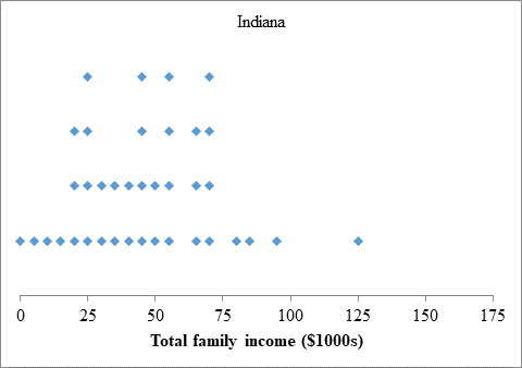
Indiana

From the above dot plot, we note that the distribution is roughly symmetric for Indiana individuals, because the peak (s) in the dot plot lies roughly in the middle of the dot plots.

We note that the peak of the distribution lies between 25 thousand dollars and 75 thousand dollars for Indiana individuals, while there is also a gap between 100 thousand dollars and 125 thousand dollars with a potential outlier at 125 thousand dollars.

The median total family income appears to be 45 thousand dollars, as this is roughly the middle value of the peak of the distribution.

Thus, the total family income in Indiana ranges from 0 to 125 thousand dollars.

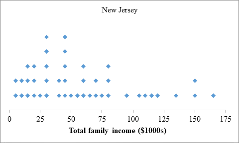
New Jersey

From the above dot plot, we note that the distribution is right-skewed for New Jersey individuals, because the peak in the dot plot lies to the left in the dot plot with a tail of less dots to the right.

We note that the single peak of the distribution lies between 25 thousand dollars and 50 thousand dollars for New Jersey individuals, while there are also a few gaps in the distribution (80-90, 100, 125-130, 155-160).

The median total family income appears to be 37.5 thousand dollars, as this is roughly the middle value of the peak of the distribution.

Thus, the total family income in New Jersey ranges from 5 thousand dollars to 165 thousand dollars.

Comparison

The distribution of Indiana individuals is roughly symmetric, while the distribution of New Jersey individuals is right-skewed.

The Indiana distribution contains a potential outlier at 125 thousand dollars, while the New Jersey distribution does not appear to contain outliers.

The median Indiana distribution appears to be slightly higher than the median of the New Jersey distribution.

The variation in the New Jersey distribution is higher than the variation in the Indiana distribution, because the spread of the dots in the dot plots is larger.