
Concept explainers
Videos
TheStreeter-Phelps model can be used to compute the dissolved oxygen concentration in a river below a point discharge of sewage (Fig. P16.17),
where
As indicated in Fig. P16.17, Eq. (P16.17) produces an oxygen “sag” that reaches a critical minimum level
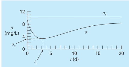
FIGURE P16.17
A dissolved oxygen “sag” below a point discharge of sewageinto a river.
below the point discharge. This point is called “critical” because it represents the locationwhere biota that depend on oxygen (like fish) would be the most stressed. Determine the critical travel time and concentration, given the following values:
Want to see the full answer?
Check out a sample textbook solution
Chapter 16 Solutions
EBK NUMERICAL METHODS FOR ENGINEERS


- The following table lists temperatures and specific volumes of water vapor at two pressures: p = 1.5 MPa v(m³/kg) p = 1.0 MPa T ("C) v(m³/kg) T ("C) 200 0.2060 200 0.1325 240 280 0.2275 0.2480 240 280 0.1483 0.1627 Data encountered in solving problems often do not fall exactly on the grid of values provided by property tables, and linear interpolation between adjacent table entries becomes necessary. Using the data provided here, estimate i. the specific volume at T= 240 °Č, p = 1.25 MPa, in m/kg ii. the temperature at p = 1.5 MPa, v = 0.1555 m/kg, in °C ii. the specific volume at T = 220 °C, p = 1.4 MPa, in m'/kgarrow_forwardCakulate the time rate of change of air density during expiration Assume that the lung (Fig. 3.11) has a total volume of 6000 ml, the diameter of the trachea is 18 mm, the airflow velocity out of the trachea is 20 cm/s, and the density of air is 1.225 kg/m. Also assume that lung volume is decreasing at a rate of 100 mL/s. Hello sir, I want the same solution, but in a detailed way and mention his data, a question, and a solution in detailing mathematics without words. Solution We will start from Eq. (3.24) because we are asked for the time rate of change of density. We are asked to find the time rate of change of air density; this suggests that Example 3.5 condis tions are representing a nonsteady flow scenario. In addition, we were told what the rate of change in the lung volume is during this procedure, further supporting the use of Eq. (3.24). pdV+ (3.24 ams Assume that at the instant in time that we are measuring the system, density is uniform within the volume of interest. This…arrow_forward9. Using simple reservoir simulation, estimate storage over time; maximum reservoir capacity is 10 volume units, and it starts full. Please a) estimate the largest spill over the simulated period, b) and the simulated storage at the beginning of 7 time step. Time Inflow Demand step (L^3) (L^3) 4 1. 10 4 2 8. 4 8. 6 7 3.arrow_forward
- Here I'm finding final kinetic energy KE2, given initial kinetic energy, initial force, alpha N/m^3 and beta N representing F(x). I integrated F(x)dx though I'm not sure how to integrate Fo with respect to X. I tried just finding the integrand ouput of 7.5x10^4m and subtracting the initial force, since the initial force would count as x=0, or I assumed. I then followed the regular approach of adding over the initial KE1 to isolate the unknown KE2 which I keeo getting as 1.07x10^10 which seems to be off. Again, I suspect where I'm going wrong is integrating the initial force -3.5x10^6N with respect to x, but other than what I've already done, that doesn't make sense to me.arrow_forwardConsider a traffic flow network of a sector of the city dependent on the parametersh and k. G00 600 a) Obtain a relation between h and k so that the corresponding system has a solution.arrow_forward1. The observed and model simulated average daily flow in month flow at the outlet of a river catchment during a given period is presented as follows. Predicted flow Observed flow 0.25 0.30 0.70 0.73 0.80 0.87 0.71 0.90 0.71 0.65 1.60 1.45 0.90 0.70 0.71 0.61 0.24 0.22 1.00 0.64 0.81 1.00 1.05 0.90 0.46 0.48 0.27 0.23 0.80 0.24 0.32 0.42 0.80 0.89 (i) Evaluate the model performance based on any two computed statistical measures of performance of your choice. (ii) Explain possible reasons for model performance observed in (i) above. (Hint: Refer to reading material provided on model evaluation by Moriasi et al., 2007)arrow_forward
- Examples 2 PPL.pdf Homework Solve the following Liner Programming Problems (LPP) which to maximize profit. Use Graphical Method Ql: Max Z= 4X1 + 3X2 S.T 5X1+3X2arrow_forwardfluid mechanics A pipe 200 (mm) diameter carries Oil at a flow rate of 0.030 (m³/s). The pipe diameter reduces from 200 (mm) to 150 (mm). Point 1 is located at the beginning of the pipe and point 2 is located at the end of the pipe. Elevation of point 1 is 165 (m) lower than elevation of point 2. Water pressure at point 2 is atmospheric pressure. Water flow in the pipe ascending from point 1 to point 2. Total head losses of flow in the pipe equals to 15 (m). 1- Find the value of pressure head of Oil at point 1. 2- Draw the H.G.L. of flow in the pipe.arrow_forward2. In class, we derived an expression for hR/RT for a gas that obeyed the Pressure Explicit Virial Expansion truncated after the third term. In class, we assumed that B and C were not functions of temperature. a. Please rework the derivation with B = B(T) and C = 0. b. Please continue the derivation under the assumption that B(T) = mT + b. Where m and b are the slope and y-intercept of a straight, respectively. %3Darrow_forward
- The SCAL results for a core sample taken from an exploration well is as follows: Capillary pressure, P (psia) Water saturation, (%) 100 Water density 64 lb/ft3 4.4 100 Oil density = 45 lb/ft3 %3D 5.3 90.1 5.6 82.4 10.5 43.7 15.7 32.2 35.0 29.8 76.5 Dementa of Reservoir Rock and Fluid Properties Ch4-Saturation and Capilary Pressure Slde 51 Exercise A P U ASIA PACInc UNIVERSITY or TECHNOLOGYA ovanoN L Convert the capillary pressure table to water saturation and height, H in ft. Plot H vs Sw. 19.5 Indicate the FWL, OWC and transition zone on the plot. LA sample was taken from a depth 80 ft above the OWC. What is the expected Sw of the sample at that elevation.arrow_forwardThe left and right water edges of a river are 2.75m and 62.45m, respectively, from an initial reference point. Verticals are located at distances 11.25, 19.25 26.75, 34.45, 40.95, 46.95, and 54.45 m, respectively from the reference point. The corresponding depths of verticals are 5.00, 9.60, 9.80, 10.00, 10.40, 10.00, and 4.80m. Mean velocities in the verticals are 0.16, 0.60, 0.75, 0.92, 0.97, 0.98, and 0.65 m/s respectively. A. Determine the Total Discharge of the river. B. Determine the average velocity of the river flow.arrow_forward3.5 Construct IPR of a well in a saturated oil reservoir using both Vogel's equation and Fetkovich's equation. The following data are given: Reservoir pressure, p = 3,500 psia Tested flowing bottom-hole 2,500 psia Tested production rate at pwf1,41 = 600 stb/day Tested flowing bottom-hole pressure, 1,500 psia Tested production rate at pwf2,42 = pressure, Pwf1 Pwf2 = 900 stb/dayarrow_forward
 Elements Of ElectromagneticsMechanical EngineeringISBN:9780190698614Author:Sadiku, Matthew N. O.Publisher:Oxford University Press
 Mechanics of Materials (10th Edition)Mechanical EngineeringISBN:9780134319650Author:Russell C. HibbelerPublisher:PEARSON
 Thermodynamics: An Engineering ApproachMechanical EngineeringISBN:9781259822674Author:Yunus A. Cengel Dr., Michael A. BolesPublisher:McGraw-Hill Education
 Control Systems EngineeringMechanical EngineeringISBN:9781118170519Author:Norman S. NisePublisher:WILEY
 Mechanics of Materials (MindTap Course List)Mechanical EngineeringISBN:9781337093347Author:Barry J. Goodno, James M. GerePublisher:Cengage Learning
 Engineering Mechanics: StaticsMechanical EngineeringISBN:9781118807330Author:James L. Meriam, L. G. Kraige, J. N. BoltonPublisher:WILEY