
Concept explainers
Videos
a.
Identify the predictors that could be used in the model to incorporate suppliers and lubrication regimens in addition to blank holder pressure.
a.
Answer to Problem 54E
The predictors that could be used in the model to incorporate suppliers and lubrication regimens in addition to blank holder pressure are given below:
Explanation of Solution
Given info:
The MINITAB output shows that the springback from the wall opening angle being predicted using blank holder pressure, three types of material suppliers and three types of lubrication regimens.
Calculation:
Dummy or indicator variable:
If there a categorical variable has k levels then k–1 dummy variables would be included in the model.
The material suppliers and lubrication regimens are categorical variables with three levels each.
For material suppliers:
Fix the third level as a base and create two dummy variables as shown below:
For lubrication regimens:
Fix the first level (no lubricant) as a base and create two dummy variables as shown below:
b.
Test the hypothesis to conclude whether the model specifies a useful relationship between springback from the wall opening angle and at least one of the five predictor variables.
b.
Answer to Problem 54E
There is sufficient evidence to conclude that the model specifies a useful relationship between the springback from the wall opening angle and at least one of the five predictor variables
Explanation of Solution
Given info:
The MINTAB output was given.
Calculation:
The test hypotheses are given below:
Null hypothesis:
That is, there is no use of linear relationship between springback from the wall opening angle and at least one of the five predictor variables.
Alternative hypothesis:
That is, there is a use of linear relationship between springback from the wall opening angle and at least one of the five predictor variables.
From the MINITAB output, it can be observed that the P-value corresponding to the F-statistic is 0.000.
Rejection region:
If
If
Conclusion:
The P- value is 0.000 and the level of significance is 0.001.
The P- value is lesser than the level of significance.
That is,
Thus, the null hypothesis is rejected,
Hence, there is sufficient evidence to conclude that there is a use of linear relationship between springback from the wall opening angle and at least one of the five predictor variables.
c.
Calculate the 95% prediction interval for the springback from the wall opening angle when BHP is 1,000, material from supplier 1 and no lubrication.
c.
Answer to Problem 54E
The 95% prediction interval for the predicted springback from the wall opening angle when BHP is 1,000, material from supplier 1 and no lubrication is
Explanation of Solution
Given info:
The BHP is 1,000, material from supplier 1 and no lubrication. The corresponding standard deviation for prediction is 0.524.
Calculation:
The prediction value of springback from the wall opening angle when BHP is 1,000, material from supplier 1 and no lubrication is calculated as follows:
Thus, the prediction value of springback from the wall opening angle when BHP is 1,000, material from supplier 1 and no lubrication is 16.4461.
95% prediction interval:
The prediction interval is calculated using the formula:
Where,
n is the total number of observations.
k is the total number of predictors in the model.
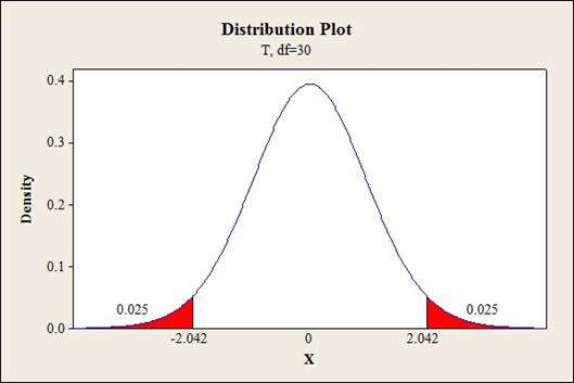
Critical value:
Software procedure:
Step-by-step procedure to find the critical value is given below:
- Click on Graph, select View Probability and click OK.
- Select t, enter 30 as Degrees of freedom, inShaded Area Tab select Probability under Define Shaded Area By and choose Both tails.
- Enter Probability value as 0.05.
- Click OK.
Output obtained from MINITAB is given below:
The 95% confidence interval for the predicted amount of beta carotene is calculated as follows:
Thus, the 95% prediction interval for the predicted springback from the wall opening angle when BHP is 1,000, material from supplier 1 and no lubricationis
d.
Find the coefficient of multiple determination.
Give the conclusion stating the importance of lubrication regimen.
d.
Answer to Problem 54E
The coefficient of multiple determination is 74.1%
The lubrication regimen is not important because there is not much of a difference in the coefficient of multiple determination even after removing the two variables corresponding to lubrication.
The two variables corresponding to lubrication shows no effect and need not be included in the model as long as the other predictors BHP and suppliers were retained.
Explanation of Solution
Given info:
The SSE after removing the variables corresponding to lubrication regimen is 48.426.
Calculation:
Coefficient of determination:
The coefficient of determination tells the total amount of variation in the dependent variable explained by the independent variable. It
Substitute 48.426 as SSE and 186.980 as SST.
Thus, the coefficient of multiple determination is 74.1%
The test hypotheses are given below:
Null hypothesis:
That is, the two dummy variables corresponding to lubrication are not significant to explain the variation in springback from wall opening angle.
Alternative hypothesis:
That is, At least one of the two dummy variables corresponding to lubrication is significant to explain the variation in springback from wall opening angle.
Test statistic:
Where,
n represents the total number of observations,
k represents the number of predictors on the full model.
l represents the number of predictors on the reduced model.
Substitute 48.426for
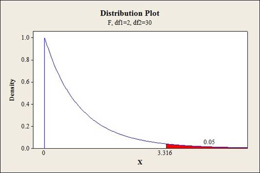
Critical value:
Software procedure:
- Click on Graph, select View Probability and click OK.
- Select F, enter 2 in numerator df and 30 in denominator df.
- Under Shaded Area Tab select Probability under Define Shaded Area By and select Right tail.
- Choose Probability value as 0.05.
- Click OK.
Output obtained from MINITAB is given below:
Conclusion:
Coefficient of determination:
The coefficient of determination for the whole model including the two variables corresponding to lubrication is 77.5% whereas the coefficient of multiple determination after removing the two variables corresponding to lubrication is 74.1%. Thus, there is a slight drop in coefficient of multiple determination.
Testing the hypothesis:
The test statistic value is 2.268 and the critical value is 3.316.
The test statistic is lesser than the critical value.
That is,
Thus, the null hypothesis is not rejected,
Hence, there is sufficient evidence to conclude thatthe two dummy variables corresponding to lubrication are not significant to explain the variation in springback from wall opening angle.
e.
Identify whether the given model has improved than the model specified in part (d).
e.
Answer to Problem 54E
Yes, the given model has improved than the model specified in part (d).
There is sufficient evidence to conclude thatthe addition of interaction terms is significant to explain the variation in springback from wall opening angle at 5% level of significance.
Explanation of Solution
Given info:
A regression model is built with the five predictors and the interactions between BHP and the four dummy variables.
The resulting SSE is 28.216 and the
Calculation:
The test hypotheses are given below:
Null hypothesis:
That is, the addition of interaction terms is not significant to explain the variation in the dependent variable y.
Alternative hypothesis:
That is, at least one of theinteraction terms is significant to explain the variation in the dependent variable y.
The degrees of freedom for the regression would be 4.
The degrees of freedom for the error would be
Test statistic:
Critical value:
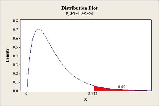
Software procedure:
- Click on Graph, select View Probability and click OK.
- Select F, enter 4 in numerator df and 26 in denominator df.
- Under Shaded Area Tab select Probability under Define Shaded Area By and select Right tail.
- Choose Probability value as 0.05.
- Click OK.
Output obtained from MINITAB is given below:
Conclusion:
The test statistic value is 3.191 and the critical value is 2.743.
The test statistic is greater than the critical value.
That is,
Thus, the null hypothesis is rejected,
Hence, there issufficient evidence to conclude thatthe addition of interaction terms is significant to explain the variation in springback from wall opening angle at 5% level of significance.
Want to see more full solutions like this?
Chapter 13 Solutions
Probability and Statistics for Engineering and the Sciences


- An article in Knee Surgery, Sports Traumatology, Arthroscopy, "Arthroscopic meniscal repair with an absorbable screw: results and surgical technique," (2005, Vol. 13, pp. 273-279) cites a success rate of 1% for meniscal tears with a rim width of less than 3 mm, and a 1% success rate for tears from 3-6 mm. If you are unlucky enough to suffer a meniscal tear of less than 3 mm on your left knee, and one of width 3-6 mm on your right knee, what is the probability that you have exactly one successful surgery? assume surgieries are independent.arrow_forwardThe article “Differences in Susceptibilities of Different Cell Lines to Bilirubin Damage” (K. Ngai, C. Yeung, and C. Leung, Journal of Paediatric Child Health, 2000:36–45) reports an investigation into the toxicity of bilirubin on several cell lines. Ten sets of human liver cells and 10 sets of mouse fibroblast cells were placed into solutions of bilirubin in albumin with a 1.4 bilirubin/albumin molar ratio for 24 hours. In the 10 sets of human liver cells, the average percentage of cells surviving was 53.9 with a standard deviation of 10.7. In the 10 sets of mouse fibroblast cells, the average percentage of cells surviving was 73.1 with a standard deviation of 9.1. Find a 98% confidence interval for the difference in survival percentages between the two cell lines.arrow_forwardThe authors of the article “Predictive Model for PittingCorrosion in Buried Oil and Gas Pipelines”(Corrosion, 2009: 332–342) provided the data on whichtheir investigation was based.a. Consider the following sample of 61 observations onmaximum pitting depth (mm) of pipeline specimensburied in clay loam soil. 0.41 0.41 0.41 0.41 0.43 0.43 0.43 0.48 0.480.58 0.79 0.79 0.81 0.81 0.81 0.91 0.94 0.941.02 1.04 1.04 1.17 1.17 1.17 1.17 1.17 1.171.17 1.19 1.19 1.27 1.40 1.40 1.59 1.59 1.601.68 1.91 1.96 1.96 1.96 2.10 2.21 2.31 2.462.49 2.57 2.74 3.10 3.18 3.30 3.58 3.58 4.154.75 5.33 7.65 7.70 8.13 10.41 13.44Construct a stem-and-leaf display in which the twolargest values are shown in a last row labeled HI.b. Refer back to (a), and create a histogram based oneight classes with 0 as the lower limit of the firstclass and class widths of .5, .5, .5, .5, 1, 2, 5, and 5,respectively.c. The accompanying comparative boxplot fromMinitab shows plots of pitting depth for four differenttypes of soils.…arrow_forward
- The propagation of fatigue cracks in various aircraft partshas been the subject of extensive study in recent years.The accompanying data consists of propagation lives(flight hours/104) to reach a given crack size in fastenerholes intended for use in military aircraft (“StatisticalCrack Propagation in Fastener Holes Under SpectrumLoading,” J. Aircraft, 1983: 1028–1032):.736 .863 .865 .913 .915 .937 .983 1.0071.011 1.064 1.109 1.132 1.140 1.153 1.253 1.394a. Compute and compare the values of the sample meanand median.b. By how much could the largest sample observationbe decreased without affecting the value of themedian?arrow_forwardLow-Birth-Weight Hospital Stays. Data on low-birthweight babies were collected over a 2-year period by 14 participating centers of the National Institute of Child Health and Human Development Neonatal Research Network. Results were reported by J. Lemons et al. in the on-line paper “Very Low Birth Weight Outcomes of the National Institute of ChildHealth and Human Development Neonatal Research Network” (Pediatrics, Vol. 107, No. 1, p. e1). For the 1084 surviving babies whose birth weights were 751– 1000 grams, the average length of stay in the hospital was 86 days, although one center had an average of 66 days and another had an average of 108 days. a. Can the mean lengths of stay be considered population means? Explain your answer.b. Assuming that the population standard deviation is 12 days, determine the z-score for a baby’s length of stay of 86 days at the center where the mean was 66 days.c. Assuming that the population standard deviation is 12 days, determine the z-score for a…arrow_forwardSuppose a researcher is interested inthe effectiveness in a new childhood exercise program implemented in a SRS of schools across a particular county. In order to test the hypothesis that the new program decreases BMI (Kg/m2), the researcher takes a SRS of children from schools where the program is employed and a SRS from schools that do not employ the program and compares the results. Assume the following table represents the SRSs of students and their BMIs. Student intervention group BMI (kg/m2) Student control group BMI (kg/m2) A 18.6 A 21.6 B 18.2 B 18.9 C 19.5 C 19.4 D 18.9 D 22.6 E 24.1 F 23.6 A) Assuming that all the necessary conditions are met (normality, independence, etc.) carry out the appropriate statistical test to determine if the new exercise program is effective. Use an alpha level of 0.05. Do not assume equal variances.B) Construct a 95% confidence interval about your estimate for the average difference in BMI between the groups.arrow_forward
- Determine the kurtosis if the data given is a sample.arrow_forwardThe article “Structural Performance of Rounded Dovetail Connections Under Different Loading Conditions” (T. Tannert, H. Prion, and F. Lam, Can J Civ Eng, 2007:1600–1605) describes a study of the deformation properties of dovetail joints. In one experiment, 10 rounded dovetail connections and 10 double rounded dovetail connections were loaded until failure. The rounded connections had an average load at failure of 8.27 kN with a standard deviation of 0.62 kN. The double-rounded connections had an average load at failure of 6.11 kN with a standard deviation of 1.31 kN. Can you conclude that the mean load at failure is greater for rounded connections than for double-rounded connections?arrow_forwardwhy is the DV female drosophila Do you use a z or test for this problem?arrow_forward
- An urban community wants to show that the incidence of breast cancer is higher in their locality than in a neighboring rural area. (PCB levels were found to be higher in the soil of the urban community). If you find that in the urban community 20 out of 200 adult women have breast cancer and that in the rural community 10 out of 150 adult women have it, could you conclude, at a significance level of 0.05, that breast cancer is more prevalent in the urban community?1. The parameter of interest is:2. The hypotheses for this test are:3. The calculated test statistic is:4. The critical region is:5. Draw the critical region (make decision):6. It can be concluded that:arrow_forwardA research on the effect of duodenal infusion of donor feces for recurrent Clostridium difficile examined patients with C. difficile infections which cause persistent diarrhea. Some patients were given the antibiotic vancomycin, while others were given a fecal transplant. At alpha = 0.01, test if the result is dependent on the type of treatment given.arrow_forwardAn article in the Journal of the Electrochemical Society (Vol. 139, No. 2, 1992, pp. 524–532) describes anexperiment to investigate the low-pressure vapor deposition of polysilicon. The experiment was carried outin a large-capacity reactor at Sematech in Austin, Texas. The reactor has several wafer positions, and fourof these positions are selected at random. The response variable is film thickness uniformity. Threereplicates of the experiment were run, and the data are as follows:a. Test the significance of these wafer position with α=0.05.b. If proven significant, perform a multiple comparison method using Fisher’s LSD.arrow_forward
 MATLAB: An Introduction with ApplicationsStatisticsISBN:9781119256830Author:Amos GilatPublisher:John Wiley & Sons Inc
 Probability and Statistics for Engineering and th...StatisticsISBN:9781305251809Author:Jay L. DevorePublisher:Cengage Learning
 Statistics for The Behavioral Sciences (MindTap C...StatisticsISBN:9781305504912Author:Frederick J Gravetter, Larry B. WallnauPublisher:Cengage Learning
 Elementary Statistics: Picturing the World (7th E...StatisticsISBN:9780134683416Author:Ron Larson, Betsy FarberPublisher:PEARSON
 The Basic Practice of StatisticsStatisticsISBN:9781319042578Author:David S. Moore, William I. Notz, Michael A. FlignerPublisher:W. H. Freeman
 Introduction to the Practice of StatisticsStatisticsISBN:9781319013387Author:David S. Moore, George P. McCabe, Bruce A. CraigPublisher:W. H. Freeman