
Introduction To Statistics And Data Analysis
6th Edition
ISBN: 9781337793612
Author: PECK, Roxy.
Publisher: Cengage Learning,
expand_more
expand_more
format_list_bulleted
Videos
Textbook Question
Chapter 5, Problem 75CR
No tortilla chip lover likes soggy chips, so it is important to find characteristics of the production process that produce chips with an appealing texture. The accompanying data on x = Frying time (in seconds) and y = Moisture content (%) appeared in the paper, “Thermal and Physical Properties of Tortilla Chips as a
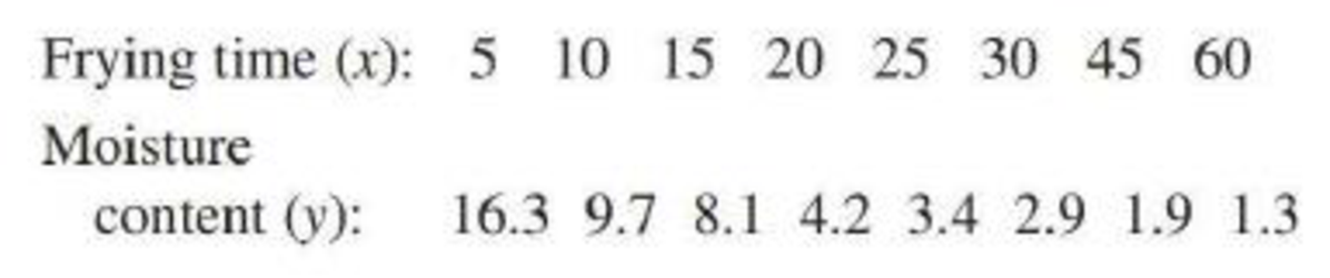
- a. Construct a
scatterplot of these data. Does the relationship between moisture content and frying time appear to be linear? - b. Transform they values using y′ = log(y) and construct a scatterplot of the (x, y′) pairs. Does this scatterplot look more nearly linear than the one in Part (a)?
- c. Find the equation of the least-squares line that describes the relationship between y′ and x.
- d. Use the least-squares line from Part (c) to predict moisture content for a frying time of 35 minutes.
Expert Solution & Answer

Trending nowThis is a popular solution!

Students have asked these similar questions
A number of studies have shown lichens (certain plants composed of an alga and a fungus) to be excellent bioindicators of air pollution. The article “The Epiphytic Lichen Hypogymnia physodes as a Biomonitor of Atmospheric Nitrogen and Sulphur Deposition in Norway” (Environ. Monitoring Assessment, 1993: 27–47) gives the following data (read from a graph) on x ¼ NO3 wet deposition (g N/m2 ) and y ¼ lichen N (% dry weight):
(refer to chart)
The author used simple linear regression to analyze the data. Use the accompanying MINITAB output to answer the following questions:
a. What are the least squares estimates of b0 and b1?
b. Predict lichen N for an NO3 deposition value of .5.
c. What is the estimate of s?
d. What is the value of total variation, and how much of it can be explained by the model relationship?
The following table gives the millions of metric tons of carbon dioxide emissions in a certain country for selected years from 2010 and projected to 2032.
Year
2010
2012
2014
2016
2018
2020
CO2 Emissions
337.5
361.5
395.1
425.8
451.1
496.4
Year
2022
2024
2026
2028
2030
2032
CO2 Emissions
558.2
592.9
628.7
662.1
709.1
742.7
(a) Create a linear function that models these data, with x as the number of years past 2010 and y as the millions of metric tons of carbon dioxide emissions. (Round all numerical values to two decimal places.)y(x) =
(b) Find the model's estimate for the 2028 data point. (Round your answer to two decimal places.) million metric tons(c) Find the slope of the linear model. (Round your answer to two decimal places.)Interpret the slope of the linear model.
For each year since ---Select--- 2009 2010 2015 2028 2032 , carbon dioxide emissions in the U.S. are expected to change by million metric tons.
An article in the Journal of Applied Polymer Science (Vol. 56, pp. 471–476, 1995) studied the effect of the mole ratio of sebacic acid on the intrinsic viscosity of copolyesters.- The data follows: Viscosity 0.45 0.2 0.34 0.58 0.7 0.57 0.55 0.44 Mole ratio 1 0.9 0.8 0.7 0.6 0.5 0.4 0.3 (a) Construct a scatter diagram of the data.
Chapter 5 Solutions
Introduction To Statistics And Data Analysis
Ch. 5.1 - For each of the scatterplots shown, answer the...Ch. 5.1 - For each of the following pairs of variables,...Ch. 5.1 - For each of the following pairs of variables,...Ch. 5.1 - For each of the following pairs of variables,...Ch. 5.1 - Is the following statement correct? Explain why or...Ch. 5.1 - Draw a scatterplot for which r = 1.Ch. 5.1 - Draw a scatterplot for which r = 1.Ch. 5.1 - Each year J.D. Power and Associates surveys new...Ch. 5.1 - The accompanying data are x = Cost (cents per...Ch. 5.1 - The authors of the paper Flat-footedness Is Not a...
Ch. 5.1 - The paper The Relationship Between Cell Phone Use,...Ch. 5.1 - Data from the U.S. Federal Reserve Board (federal...Ch. 5.1 - The article 115K! The 13 Best Paying U.S....Ch. 5.1 - It may seem odd, but one of the ways biologists...Ch. 5.1 - An auction house released a list of 25 recently...Ch. 5.1 - A sample of automobiles traversing a certain...Ch. 5.2 - Two scatterplots are shown below. Explain why it...Ch. 5.2 - The authors of the paper Statistical Methods for...Ch. 5.2 - The accompanying data are a subset of data from...Ch. 5.2 - The authors of the paper Evaluating Existing...Ch. 5.2 - The authors of the paper referenced in the...Ch. 5.2 - A sample of 548 ethnically diverse students from...Ch. 5.2 - The relationship between hospital patient-to-nurse...Ch. 5.2 - The report Airline Quality Rating 2016...Ch. 5.2 - Acrylamide is a chemical that is sometimes found...Ch. 5.2 - Use the acrylamide data given in the previous...Ch. 5.2 - Studies have shown that people who suffer sudden...Ch. 5.2 - The data given in the previous exercise on x =...Ch. 5.2 - An article on the cost of housing in Califomia...Ch. 5.2 - The following data on sale price, size, and...Ch. 5.2 - Explain why it can be dangerous to use the...Ch. 5.2 - The sales manager of a large company selected a...Ch. 5.2 - Explain why the slope b of the least-squares line...Ch. 5.2 - Prob. 34ECh. 5.3 - Does it pay to stay in school? The report Trends...Ch. 5.3 - The data in the accompanying table is from the...Ch. 5.3 - The paper referenced in the previous exercise also...Ch. 5.3 - Consider the residual plot from the previous...Ch. 5.3 - The report Airline Quality Rating 2016...Ch. 5.3 - Acrylamide is a chemical that is sometimes found...Ch. 5.3 - Consider the scatterplot of acrylamide...Ch. 5.3 - Some types of algae have the potential to cause...Ch. 5.3 - The relationship between x = Total number of...Ch. 5.3 - The residuals from the least-squares line for the...Ch. 5.3 - The first Batman movie was made over 50 years ago...Ch. 5.3 - The article 115K! The 13 Best Paying U.S....Ch. 5.3 - The article Examined Life: What Stanley H. Kaplan...Ch. 5.3 - The accompanying data are a subset of data from...Ch. 5.3 - The article California State Parks Closure List...Ch. 5.3 - The article referenced in the previous exercise...Ch. 5.3 - A study was carried out to investigate the...Ch. 5.3 - Both r2 and se are used to assess the fit of a...Ch. 5.3 - Prob. 53ECh. 5.4 - The following data on x = Frying time (in seconds)...Ch. 5.4 - Use the information provided in the previous...Ch. 5.4 - The paper Aspects of Food Finding by Wintering...Ch. 5.4 - Food intake of grazing animals is limited by the...Ch. 5.4 - A study, described in the paper Prediction of...Ch. 5.4 - Prob. 59ECh. 5.4 - The following table gives the number of heart...Ch. 5.4 - Refer to the heart transplant data given in the...Ch. 5.4 - The paper Population Pressure and Agricultural...Ch. 5.4 - Determining the age of an animal can sometimes be...Ch. 5.5 - The paper How Lead Exposure Relates to Temporal...Ch. 5.5 - The following quote is from the paper Evaluation...Ch. 5 - The accompanying data represent x = Amount of...Ch. 5 - The paper A Cross-National Relationship Between...Ch. 5 - The following data on x = Score on a measure of...Ch. 5 - The paper Effects of Canine Parvovirus (CPV) on...Ch. 5 - The paper Depression, Body Mass Index, and Chronic...Ch. 5 - The paper Aspects of Food Finding by Wintering...Ch. 5 - Data on salmon availability (x) and the percentage...Ch. 5 - No tortilla chip lover likes soggy chips, so it is...Ch. 5 - The article Reduction is Soluble Protein and...Ch. 5 - The following quote is from the paper The Weight...Ch. 5 - An accurate assessment of oxygen consumption...Ch. 5 - Consider the four (x, y) pairs (0, 0), (1, 1), 1,...Ch. 5 - Prob. 1CRECh. 5 - Data from a survey of 1046 adults age 50 and older...Ch. 5 - Prob. 3CRECh. 5 - Prob. 4CRECh. 5 - Prob. 5CRECh. 5 - The amount of money spent each year on science,...Ch. 5 - Below are the data used to construct the time...Ch. 5 - In August 2009, Harris Interactive released the...Ch. 5 - Prob. 9CRECh. 5 - Prob. 10CRECh. 5 - Prob. 11CRECh. 5 - Prob. 12CRECh. 5 - Cost-to-charge ratios (the percentage of the...Ch. 5 - In the article Reproductive Biology of the Aquatic...Ch. 5 - Prob. 15CRECh. 5 - Anabolic steroid abuse has been increasing despite...Ch. 5 - Prob. 81ECh. 5 - Prob. 82ECh. 5 - Prob. 83ECh. 5 - Prob. 84ECh. 5 - Suppose the hypothetical data below are from a...Ch. 5 - Prob. 86E
Additional Math Textbook Solutions
Find more solutions based on key concepts
(a) For each data set, find the mean, median, and mode. (b) Discuss anything about the data that affects the us...
APPLIED STAT.IN BUS.+ECONOMICS
the type of variable is the response.
Stats: Modeling the World Nasta Edition Grades 9-12
Ten equally qualified marketing assistants are candidates for promotion to associate buyer; seven are men and t...
An Introduction to Mathematical Statistics and Its Applications (6th Edition)
Empirical versus Theoretical A Monopoly player claims that the probability of getting a 4 when rolling a six-si...
Introductory Statistics (2nd Edition)
Use the model developed in Example 1.5 to predict the total sales for weeks 2 through 16, and compare the resul...
Business Analytics
10. Explain the steps in designing an experiment.
Fundamentals of Statistics (5th Edition)
Knowledge Booster


Learn more about
Need a deep-dive on the concept behind this application? Look no further. Learn more about this topic, statistics and related others by exploring similar questions and additional content below.Similar questions
- An article in Technometrics (1974, Vol. 16, pp. 523–531) considered the following stack-loss data from a plant oxidizing ammonia to nitric acid. Twenty-one daily responses of stack loss (the amount of ammonia escaping) were measured with air flow x1, temperature x2, and acid concentration x3. y = 42, 37, 37, 28, 18, 18, 19, 20, 15, 14, 14, 13, 11, 12, 8, 7, 8, 8, 9, 15, 15 x1 = 80, 80, 75, 62, 62, 62, 62, 62, 58, 58, 58, 58, 58, 58, 50, 50, 50, 50, 50, 56, 70 x2 = 27, 27, 25, 24, 22, 23, 24, 24, 23, 18, 18, 17, 18, 19, 18, 18, 19, 19, 20, 20, 20 x3 = 89, 88, 90, 87, 87, 87, 93, 93, 87, 80, 89, 88, 82, 93, 89, 86, 72, 79, 80, 82, 91 (a) Fit a linear regression model relating the results of the stack loss to the three regressor variables. (b) Estimate σ2. (c) Find the standard error se(βj). (d) Use the model in part (a) to predict stack loss when x1 = 60, x2 = 26, and x3 = 85.arrow_forwardSnowpacks contain a wide spectrum of pollutants thatmay represent environmental hazards. The article“Atmospheric PAH Deposition: Deposition Velocitiesand Washout Ratios” (J. of EnvironmentalEngineering, 2002: 186–195) focused on the depositionof polyaromatic hydrocarbons. The authors proposeda multiple regression model for relating depositionover a specified time period (y, in mg/m2) to tworather complicated predictors x1 (mg-sec/m3) and x2 (mg/m2), defined in terms of PAH air concentrations forvarious species, total time, and total amount of precipitation.Here is data on the species fluoranthene andcorresponding Minitab output:obs x1 x2 flth1 92017 .0026900 278.782 51830 .0030000 124.533 17236 .0000196 22.654 15776 .0000360 28.685 33462 .0004960 32.666 243500 .0038900 604.707 67793 .0011200 27.698 23471 .0006400 14.189 13948 .0004850 20.6410 8824 .0003660 20.6011 7699 .0002290 16.6112 15791 .0014100 15.0813 10239 .0004100 18.0514 43835 .0000960 99.7115 49793 .0000896 58.9716 40656…arrow_forwardThe chief economist for Argus Corporation, a large appliance manufacturer, estimated the firm’s short-run cost function for vacuum cleaners using an average variable cost function of the form AVC = a + bQ + cQ2 where AVC = dollars per vacuum cleaner and Q = number of vacuum cleaners produced each month. Total fixed cost each month is $180,000. The following results were obtained: DEPENDENT VARIABLE: AVC R-SQUARE F-RATIO P-VALUE ON F OBSERVATIONS: 19 0.7360 39.428 0.0001 VARIABLE PARAMETER ESTIMATE STANDARD ERROR T-RATIO P-VALUE INTERCEPT 191.93 54.65 3.512 0.0029 Q -0.0305 0.00789 23.866 0.0014 Q2 0.0000024 0.00000098 2.449 0.0262 c) If Argus Corporation produces 8,000 vacuum cleaners per month, what is the Marginal cost?arrow_forward
- The chief economist for Argus Corporation, a large appliance manufacturer, estimated the firm’s short-run cost function for vacuum cleaners using an average variable cost function of the form AVC = a + bQ + cQ2 where AVC = dollars per vacuum cleaner and Q = number of vacuum cleaners produced each month. Total fixed cost each month is $180,000. The following results were obtained: DEPENDENT VARIABLE: AVC R-SQUARE F-RATIO P-VALUE ON F OBSERVATIONS: 19 0.7360 39.428 0.0001 VARIABLE PARAMETER ESTIMATE STANDARD ERROR T-RATIO P-VALUE INTERCEPT 191.93 54.65 3.512 0.0029 Q -0.0305 0.00789 23.866 0.0014 Q2 0.0000024 0.00000098 2.449 0.0262 f) At what level of output will average variable cost be at a minimum?arrow_forwardThe chief economist for Argus Corporation, a large appliance manufacturer, estimated the firm’s short-run cost function for vacuum cleaners using an average variable cost function of the form AVC = a + bQ + cQ2 where AVC = dollars per vacuum cleaner and Q = number of vacuum cleaners produced each month. Total fixed cost each month is $180,000. The following results were obtained: DEPENDENT VARIABLE: AVC R-SQUARE F-RATIO P-VALUE ON F OBSERVATIONS: 19 0.7360 39.428 0.0001 VARIABLE PARAMETER ESTIMATE STANDARD ERROR T-RATIO P-VALUE INTERCEPT 191.93 54.65 3.512 0.0029 Q -0.0305 0.00789 23.866 0.0014 Q2 0.0000024 0.00000098 2.449 0.0262 c) If Argus Corporation produces 8,000 vacuum cleaners per month, what is the estimated average variable cost?arrow_forwardThe table below shows (lifetime) peptic ulcer rates (per 100 population), UU, for various family incomes, xx, as reported by the 1989 National Health Interview Survey. Income 4000 6000 8000 12000 16000 20000 30000 45000 60000 Ulcer rate 14.1 13.1 13.8 12.6 11.8 11.7 11.5 9.3 7.6 (a) Find the equation of the regression line. Ulcer rate, U(x)= . (b) Estimate the peptic ulcer rate for an income level of x0= 25000 according to the linear model in part (a). Ulcer rate, U(x0)= .arrow_forward
- A researcher hypothesizes that in a certain country the net annual growth of private sector purchases of government bonds, B, is positively related to the nominal rate of interest on the bonds, NI, and negatively related to the rate of inflation Π: Bt = a0 + a1NIt + a2Π t + ut Note that it may be hypothesized that B depends on the real rate of interest on bonds, R, where R = NI – Π. Using a sample of 56 annual observations, s/he estimates the following equations: (1) Bt = 0.43 + 0.90NIt - 0.97Πt R21 = 0.962, SSR1 = 2.20, QRESET(F1,52) = 16.6 (3.58) (8.80) (-1.05) (2) Bt = 0.44 + 0.94Rt R22 = 0.960, SSR2 = 2.22, QRESET(F1,53) = 0.9 (9.70) (16.7) (3) Bt = 0.44 + 1.14NIt SSR3 = 9.20, QRESET(F1,53) = 59.9 (8.84) (36.1) (4) NIt = 0.08 + 0.94Πt R24 = 0.997, SSR4 = 0.18, QRESET(F1,53) = 1.4…arrow_forwardThe following regression model describes the relation between the number of days of experience in a job involving the wiring of electronic components and the number of components which were rejected stack N u m b e r space o f space r e j e c t s with hat on top equals 249 minus 1.4 space D a y s space o f space e x p e r i e n c e Based on this model, estimate the number of components rejected for an employee with 97 days of experience in the job. Round your answer to one decimal place.arrow_forwardThe following partial JMP regression output for the Fresh detergent data relates to predicting demand for future sales periods in which the price difference will be .10. SE Fit = .165360573, s = .628152. Predicted Demand Lower 95% MeanDemand Upper 95% MeanDemand 31 8.181072245 7.842346262 8.519798229 StdErr IndivDemand Lower 95% IndivDemand Upper 95% MeanDemand 0.649552965 6.850522511 9.511621980 Click here for the Excel Data File (a) Report a point estimate of and a 95 percent confidence interval for the mean demand for Fresh in all sales periods when the price difference is .10. (Round your CI answers to 3 decimal places and other answer to 4 decimal places.) (b) Report a point prediction of and a 95 percent prediction interval for the actual demand for Fresh in an individual sales period when the price difference is .10. (Round your PI answers to 3 decimal places and other answer to 4 decimal places.) (c) StdErr Indiv Demand on…arrow_forward
- The table below contains the average public school classroom teacher's salaries, , for an 11-year period. Letting represent 1990, use a graphing utility to find a linear model for the data. Year 1990 1991 1992 1993 1994 1995 Salary 32669 33462 35288 35692 37007 36266 Year 1996 1997 1998 1999 2000 Salary 37004 40108 41236 41937 43676 Salary, written as a function of is given byarrow_forwardThe following table gives the quantity demanded of ice cream (Qic) in kgs per year in Sardinia (Italy), its price (Pic) in $ per kg, consumers’ income (I) in $, the temperature (T) in Celsius, and the price of cappuccino (Pc) in $ per kg: Year Qic Pic ($/kg) I ($) T Pc ($/kg) 2000 72000 11 2000 20 14 2001 81000 10 2100 24 15 2002 90000 9 2200 25 15 2003 99000 7 2305 26 16 2004 108000 6 2407 30 17 2005 126000 4 2500 32 18 2006 117000 7 2610 26 16 2007 117000 8 2698 25 16 2008 135000 5 2801 31 18 2009 135000 5 2921 31 18 2010 144000 4 3000 34 20 2011 180000 2 3099 36 21 2012 162000 5 3201 33 19 2013 171000 4 3308 35 21 2014 153000 6 3397 30 18 2015 180000 3 3501 35 22 2016 171000 4 3689 33 20 2017 180000 3 3800 36 23…arrow_forwardThe following table gives the quantity demanded of ice cream (Qic) in kgs per year in Sardinia (Italy), its price (Pic) in $ per kg, consumers’ income (I) in $, the temperature (T) in Celsius, and the price of cappuccino (Pc) in $ per kg: Year Qic Pic ($/kg) I ($) T Pc ($/kg) 2000 72000 11 2000 20 14 2001 81000 10 2100 24 15 2002 90000 9 2200 25 15 2003 99000 7 2305 26 16 2004 108000 6 2407 30 17 2005 126000 4 2500 32 18 2006 117000 7 2610 26 16 2007 117000 8 2698 25 16 2008 135000 5 2801 31 18 2009 135000 5 2921 31 18 2010 144000 4 3000 34 20 2011 180000 2 3099 36 21 2012 162000 5 3201 33 19 2013 171000 4 3308 35 21 2014 153000 6 3397 30 18 2015 180000 3 3501 35 22 2016 171000 4 3689 33 20 2017 180000 3 3800 36 23…arrow_forward
arrow_back_ios
SEE MORE QUESTIONS
arrow_forward_ios
Recommended textbooks for you
 Algebra & Trigonometry with Analytic GeometryAlgebraISBN:9781133382119Author:SwokowskiPublisher:Cengage
Algebra & Trigonometry with Analytic Geometry
Algebra
ISBN:9781133382119
Author:Swokowski
Publisher:Cengage
Hypothesis Testing using Confidence Interval Approach; Author: BUM2413 Applied Statistics UMP;https://www.youtube.com/watch?v=Hq1l3e9pLyY;License: Standard YouTube License, CC-BY
Hypothesis Testing - Difference of Two Means - Student's -Distribution & Normal Distribution; Author: The Organic Chemistry Tutor;https://www.youtube.com/watch?v=UcZwyzwWU7o;License: Standard Youtube License