Videos
An experiment was conducted to examine the influence of avian pancreatic polypeptide (aPP), cholecystokinin (CCK), vasoactive intestinal peptide (VIP), and secretin on pancreatic
and biliary secretions in laying hens. In particular, researchers were concerned with the extent to which these hormones increase or decrease biliary and pancreatic flows and their pH values.
White leghorn hens, 14−29 weeks of age, were surgically fitted with cannulas for collecting pancreatic and biliary secretions and a jugular cannula for continuous infusion of aPP, CCK, VIP, or secretin. One trial per day was conducted on a hen, as long as her implanted cannulas remained
Each trial began with infusion of physiologic saline for 20 minutes. At the end of this period, pancreatic and biliary secretions were collected and the cannulas were attached to new vials. The biliary and pancreatic flow rates (in microliters per minute) and pH values (if possible) were measured. Infusion of a hormone was then begun and continued for 40 minutes. Measurements were then repeated.
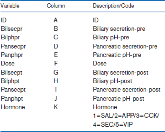
Data Set HORMONE.DAT (at www.cengagebrain com) contains data for the four hormones and saline, where saline indicates trials in which physiologic saline was infused in place of an active hormone during the second period. Each trial is one record in the file. There are 11 variables associated with each trial, as shown in Table 8.22.
Table 8.22 Format of HORMONE.DAT
Assess whether there are significant changes in secretion rates or pH levels with any of the hormones or with saline.
Want to see the full answer?
Check out a sample textbook solution
Chapter 8 Solutions
Fundamentals of Biostatistics


- A paper investigated the driving behavior of teenagers by observing their vehicles as they left a high school parking lot and then again at a site approximately 1 2 mile from the school. Assume that it is reasonable to regard the teen drivers in this study as representative of the population of teen drivers. MaleDriver FemaleDriver 1.4 -0.2 1.2 0.5 0.9 1.1 2.1 0.7 0.7 1.1 1.3 1.2 3 0.1 1.3 0.9 0.6 0.5 2.1 0.5 (a) Use a .01 level of significance for any hypothesis tests. Data consistent with summary quantities appearing in the paper are given in the table. The measurements represent the difference between the observed vehicle speed and the posted speed limit (in miles per hour) for a sample of male teenage drivers and a sample of female teenage drivers. (Use ?males − ?females. Round your test statistic to two decimal places. Round your degrees of freedom down to the nearest whole number. Round your p-value to three decimal places.) t = df =…arrow_forwardA paper investigated the driving behavior of teenagers by observing their vehicles as they left a high school parking lot and then again at a site approximately 1 2 mile from the school. Assume that it is reasonable to regard the teen drivers in this study as representative of the population of teen drivers. MaleDriver FemaleDriver 1.3 -0.3 1.3 0.6 0.9 1.1 2.1 0.7 0.7 1.1 1.3 1.2 3 0.1 1.3 0.9 0.6 0.5 2.1 0.5 (a) Use a .01 level of significance for any hypothesis tests. Data consistent with summary quantities appearing in the paper are given in the table. The measurements represent the difference between the observed vehicle speed and the posted speed limit (in miles per hour) for a sample of male teenage drivers and a sample of female teenage drivers. (Use ?males − ?females. Round your test statistic to two decimal places. Round your degrees of freedom down to the nearest whole number. Round your p-value to three decimal places.) t = df =…arrow_forwardConsider a cohort study to compare the mortality rate of myocardial infarction (MI) in men with sedentary work (exposed group) to men with physically active work (unexposed). If in the exposed, there were 36,000 person (man) years of observation and 126 deaths whereas the unexposed had 24,000 man-years of observation and 44 deaths. Compute the following a) Mortality rate in each cohort? b) What is the relative risk of dying, comparing these 2 groups? c) What is the attributable risk of sedentary work? d) What is the attributable benefit of physical activity? e) If we assume that MI is associated with the mortality in this cohort (causality), what proportion of the disease in the higher group is potentially preventable?arrow_forward
- The article “Effects of Diets with Whole Plant-Origin Proteins Added with Different Ratiosof Taurine:Methionine on the Growth, Macrophage Activity and Antioxidant Capacity ofRainbow Trout (Oncorhynchus mykiss) Fingerlings” (O. Hernandez, L. Hernandez, et al.,Veterinary and Animal Science, 2017:4-9) reports that a sample of 210 juvenile rainbowtrout fed a diet fortified with equal amounts of the amino acids taurine and methionine for aperiod of 70 days had a mean weight gain of 313 percent with a standard deviation of 25, while 210 fish fed with a control diet had a mean weight gain of 233 percent with a standard deviation of 19. Units are percent. Find a 99% confidence interval for the difference in weight gain on the two diets.arrow_forwardA research was conducted which revealed that the students’ usage of mobile phones has nowadays increased after the pandemic due to online classes and submission of their assignments and quizzes. Already the usage of mobile phones for the students was growing due to social media and different online games. The data of 25 students is provided to you in Table 2.1 that displays hours (time) spend by the children on mobile phones per week. Table 2.1 67 64 59 66 59 68 64 61 65 67 67 67 63 59 65 69 62 70 70 60 59 65 66 69 67 You are required to Compute the Frequency Distribution, Cumulative Frequency and Cumulative Relative Frequency. Sketch Histogram in Excel. Define the skewness of the drawn Histogram.arrow_forwardIn a study of exhaust emissions from school buses, the pollution intake by passengers was determined for a sample of nine school buses used in the Southern California Air Basin. The pollution intake is the amount of exhaust emissions, in grams per person per million grams emitted, that would be inhaled while traveling on the bus during its usual 18-mile18-mile trip on congested freeways from South Central LA to a magnet school in West LA. (In comparison, a city of 11 million people will inhale a total of about 1212 grams of exhaust per million grams emitted.) The amounts for the nine buses when driven with the windows open are given in the table. 1.15 0.33 0.40 0.33 1.35 0.38 0.25 0.40 0.35 A good way to judge the effect of outliers is to do your analysis twice, once with the outliers and a second time without them. Give the 90%90% confidence interval with all the data for the mean pollution intake among all school buses used in the Southern California Air Basin that…arrow_forward
- Here is a dataset containing plant growth measurements of plants grown in solutions of commonly-found chemicals in roadway runoff.Phragmites australis, a fast-growing non-native grass common to roadsides and disturbed wetlands of Tidewater Virginia, was grown in a greenhouse and watered with either: Distilled water (control); A weak petroleum solution (representing standard roadway runoff); Sodium chloride solution; Magnesium chloride solution; De-icing brine (50% sodium chloride and 50% magnesium chloride).Twenty grass preparations were used for each solution, and total growth (in cm) was recorded after watering every other day for 40 days.-Perform the correct statistical test to determine the p-value.-Report your answer rounded to four decimal places.-You should use formulas, functions, and the Data Analysis ToolPak in MS Excel to avoid additive rounding errors. Here are some useful functions: =t.test(array1,array2,tails,type) Produces a p-value for any…arrow_forwardIn a classic study, Shrauger (1972) examined the effect of an audience on performance for two groups of participants: high self-esteem and low self-esteem individuals. The participants in the study were given a problem-solving task with half of the individuals in each group working alone and a half working with an audience. Performance on the problem-solving task was measured for each individual. The results showed that the presence of an audience had little effect on high self-esteem participants but significantly lowered the performance for the low self-esteem participants. a. How many factors does this study have? What are they? b. Describe this study using the notation system that indicates factors and numbers of levels of each factor.arrow_forwardA paper investigated the driving behavior of teenagers by observing their vehicles as they left a high school parking lot and then again at a site approximately 1 2 mile from the school. Assume that it is reasonable to regard the teen drivers in this study as representative of the population of teen drivers. Amount by Which Speed Limit Was Exceeded MaleDriver FemaleDriver 1.2 -0.1 1.4 0.4 0.9 1.1 2.1 0.7 0.7 1.1 1.3 1.2 3 0.1 1.3 0.9 0.6 0.5 2.1 0.5 (a) Use a .01 level of significance for any hypothesis tests. Data consistent with summary quantities appearing in the paper are given in the table. The measurements represent the difference between the observed vehicle speed and the posted speed limit (in miles per hour) for a sample of male teenage drivers and a sample of female teenage drivers. (Use μmales − μfemales.Round your test statistic to two decimal places. Round your degrees of freedom down to the nearest whole number. Round your p-value to…arrow_forward
- A paper investigated the driving behavior of teenagers by observing their vehicles as they left a high school parking lot and then again at a site approximately 1 2 mile from the school. Assume that it is reasonable to regard the teen drivers in this study as representative of the population of teen drivers. Amount by Which Speed Limit Was Exceeded MaleDriver FemaleDriver 1.3 -0.1 1.3 0.4 0.9 1.1 2.1 0.7 0.7 1.1 1.3 1.2 3 0.1 1.3 0.9 0.6 0.5 2.1 0.5 (a) Use a .01 level of significance for any hypothesis tests. Data consistent with summary quantities appearing in the paper are given in the table. The measurements represent the difference between the observed vehicle speed and the posted speed limit (in miles per hour) for a sample of male teenage drivers and a sample of female teenage drivers. (Use μmales − μfemales.Round your test statistic to two decimal places. Round your degrees of freedom down to the nearest whole number. Round your p-value to…arrow_forwardSuppose that the index model for two Canadian stocks HD and ML is estimated with the following results: RHD =-0.03+2.10RM+eHD R-squared =0.7 RML =0.06+1.60RM+eML R-squared =0.6 σM =0.15 where M is S&P/TSX Comp Index and RX is the excess return of stock X. What is the covariance and the correlation coefficient between HD and ML?arrow_forwardA U.S. Food Survey showed that Americans routinely eat beef in their diet. Suppose that in a study of 49 consumers in Illinois and 64 consumers in Texas the following results were obtained from two samples regarding average yearly beef consumption: Illinois Texas = 49 = 64 = 54.1lb = 60.4lb S1 = 7.0 S2 = 8.0 Formulate a hypothesis so that, if the null hypothesis is rejected, we can conclude that the average amount of beef eaten annually by consumers in Illinois is significantly less than that eaten by consumers in Texas.arrow_forward
 Glencoe Algebra 1, Student Edition, 9780079039897...AlgebraISBN:9780079039897Author:CarterPublisher:McGraw Hill