
Concept explainers
Videos
a.
Justify whether the transformation
a.
Answer to Problem 59E
The transformation
Explanation of Solution
Calculation:
Reference: Exercise 5.58: The data on success (%), y and energy of shock, x is given.
The suitable transformation can be identified by constructing
Consider the transformed variable,
Data transformation
Software procedure:
Step-by-step procedure to transform the data using MINITAB software is given below:
- Choose Calc > Calculator.
- Enter the column of sqrt(x) under Store result in variable.
- Enter the formula SQRT(‘x’) under Expression.
- Click OK.
The transformed variable is stored in the column sqrt(x).
Scatterplot:
Software procedure:
Step-by-step procedure to draw the scatterplot using MINITAB software is given below:
- Choose Graph > Scatterplot.
- Choose Simple, and then click OK.
- Enter the column of y under Y variables.
- Enter the column of sqrt(x) under X variables.
- Click OK.
The output obtained using MINITAB is as follows:
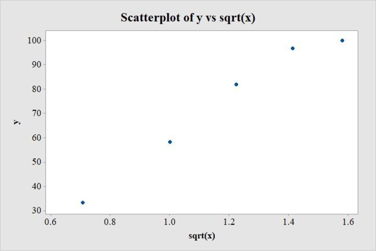
Consider the transformed variable,
Data transformation
Software procedure:
Step-by-step procedure to transform the data using MINITAB software is given below:
- Choose Calc > Calculator.
- Enter the column of sqrt(x) under Store result in variable.
- Enter the formula LN(‘x’) under Expression.
- Click OK.
The transformed variable is stored in the column ln(x).
Scatterplot:
Software procedure:
Step-by-step procedure to draw the scatterplot using MINITAB software is given below:
- Choose Graph > Scatterplot.
- Choose Simple, and then click OK.
- Enter the column of y under Y variables.
- Enter the column of ln(x) under X variables.
- Click OK.
The output obtained using MINITAB is as follows:
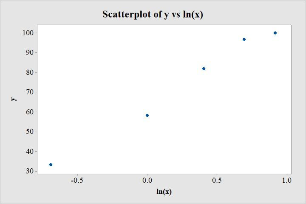
A careful observation of the scatterplot between y and
On the other hand, the scatterplot between y and
Thus, the transformation
b.
Find the least-squares regression line between y and the transformation recommended in the previous part.
b.
Answer to Problem 59E
The least-squares regression equation between y and the transformation recommended in the previous part, that is,
Explanation of Solution
Calculation:
Regression:
Software procedure:
Step by step procedure to get regression equation using MINITAB software is given as,
- Choose Stat > Regression > Regression > Fit Regression Model.
- Under Responses, enter the column of y.
- Under Continuous predictors, enter the columns of ln(x).
- Choose Results and select Analysis of Variance, Model Summary, Coefficients, Regression Equation.
- Click OK on all dialogue boxes.
The outputs using MINITAB software is given as follows:
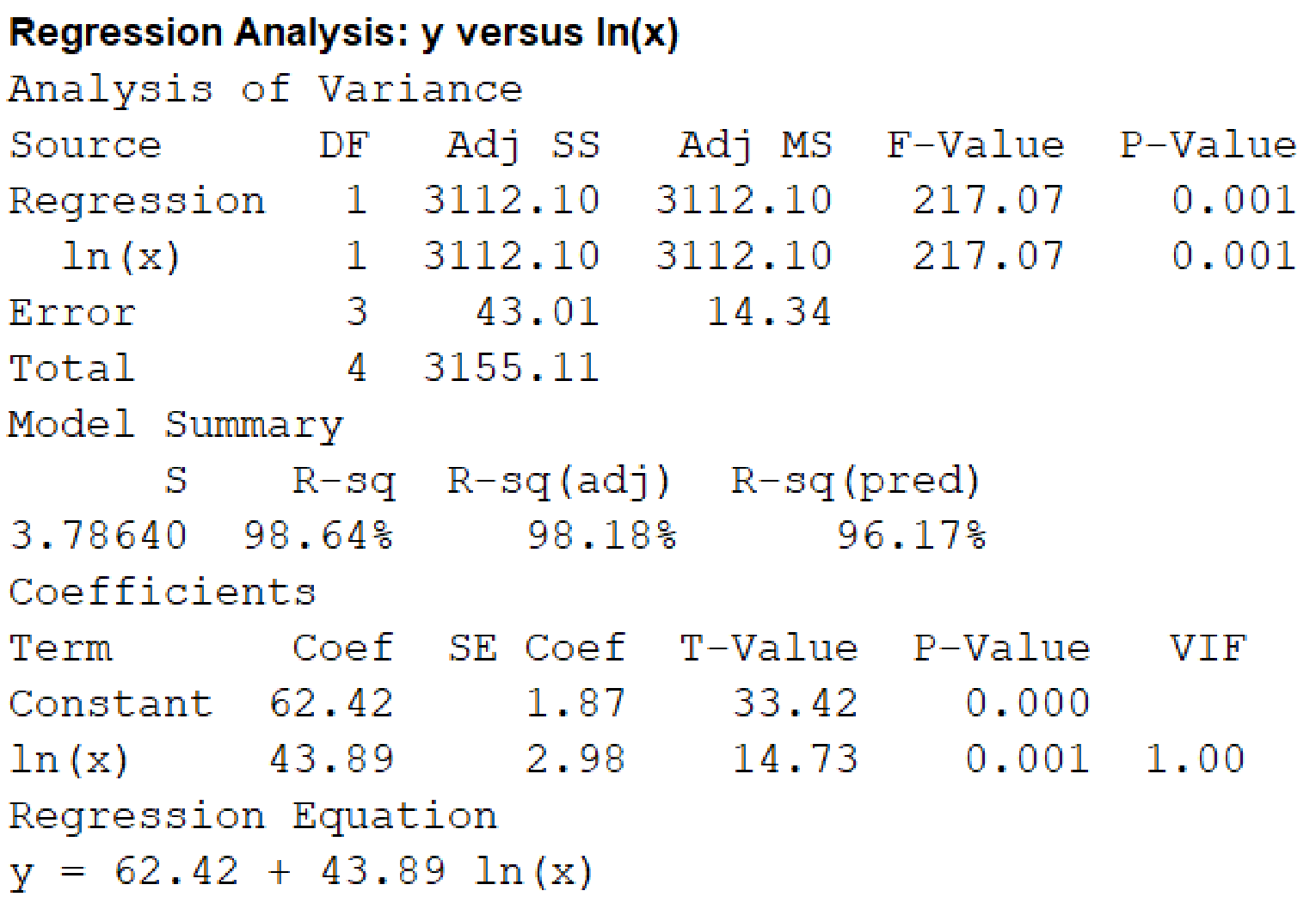
From the output, the least-squares regression equation between y and the transformation recommended in the previous part, that is,
c.
Predict the success for an energy shock 1.75 times the threshold.
Predict the success for an energy shock 0.8 times the threshold.
c.
Answer to Problem 59E
The success for an energy shock 1.75 times the threshold is 86.98%.
The success for an energy shock 0.8 times the threshold is 52.63%.
Explanation of Solution
Calculation:
The energy of shock is given as a multiple of the threshold of defibrillation.
For an energy shock 1.75 times the threshold,
Thus, the success for an energy shock 1.75 times the threshold is 86.98%.
For an energy shock 0.8 times the threshold,
Thus, the success for an energy shock 0.8 times the threshold is 52.63%.
Want to see more full solutions like this?
Chapter 5 Solutions
Introduction To Statistics And Data Analysis


- Find the equation of the regression line for the following data set. x 1 2 3 y 0 3 4arrow_forwardFor the following exercises, consider the data in Table 5, which shows the percent of unemployed ina city of people 25 years or older who are college graduates is given below, by year. 40. Based on the set of data given in Table 6, calculate the regression line using a calculator or other technology tool, and determine the correlation coefficient to three decimal places.arrow_forwardFor the following exercises, consider this scenario: The profit of a company decreased steadily overa ten-year spam.The following ordered pairs shows dollars and the number of units sold in hundreds and the profit in thousands ofover the ten-year span, (number of units sold, profit) for specific recorded years: (46,600),(48,550),(50,505),(52,540),(54,495). Use linear regression to determine a function Pwhere the profit in thousands of dollars depends onthe number of units sold in hundreds.arrow_forward
- For the following exercises, consider the data in Table 5, which shows the percent of unemployed in a city ofpeople25 years or older who are college graduates is given below, by year. 41. Based on the set of data given in Table 7, calculatethe regression line using a calculator or othertechnology tool, and determine the correlationcoefficient to three decimal places.arrow_forwardThe population Pinmillions of Texas from 2001 through 2014 can be approximated by the model P=20.913e0.0184t, where t represents the year, with t=1 corresponding to 2001. According to this model, when will the population reach 32 million?arrow_forwardOlympic Pole Vault The graph in Figure 7 indicates that in recent years the winning Olympic men’s pole vault height has fallen below the value predicted by the regression line in Example 2. This might have occurred because when the pole vault was a new event there was much room for improvement in vaulters’ performances, whereas now even the best training can produce only incremental advances. Let’s see whether concentrating on more recent results gives a better predictor of future records. (a) Use the data in Table 2 (page 176) to complete the table of winning pole vault heights shown in the margin. (Note that we are using x=0 to correspond to the year 1972, where this restricted data set begins.) (b) Find the regression line for the data in part ‚(a). (c) Plot the data and the regression line on the same axes. Does the regression line seem to provide a good model for the data? (d) What does the regression line predict as the winning pole vault height for the 2012 Olympics? Compare this predicted value to the actual 2012 winning height of 5.97 m, as described on page 177. Has this new regression line provided a better prediction than the line in Example 2?arrow_forward
- Solve the following problems completely. An article in the Journal of Environmental Engineering (1989, Vol. 115(3), reported the results of a study on the occurrence of sodium and chloride in surface streams in central Rhode Island. The following data are chloride concentration y (in milligrams per liter) and roadway area in the watershed x (in percentage). Draw a scatter diagram of the data. Fit the simple linear regression model using the method of least squares. Find an estimate of σ2. Estimate the mean chloride concentration for a watershed that has 1% roadway area. Find the fitted value corresponding to x = 0.47 and the associated residual. Test the hypothesis H0: β1 = 0 versus H1: β1 ≠ 0 using the analysis of variance procedure with α = 0.01. Find a 99% confidence interval of Mean chloride concentration when roadway area x = 1.0% Find a 99% prediction interval on chloride concentration when roadway area x = 1.0%. Plot the residuals versus ŷ and versus x. Interpret these plots.…arrow_forward1) Find the regression equation and r value Drop Height, y (m) Square of Mean Fall time, t^2 (s^2) 0.100 0.0188 0.300 0.0576 0.500 0.0980 1.000 0.198 1.500 0.305 2.500 0.508arrow_forwardA researcher conducted a number of descriptive statistics for two variables X and Y. They were as follows: SP = -20; SSx = 4; My = 7; Mx = 3 What is b equal to? What is a equal to? Using b and a construct a regression equation, and then using the regression equation, calculate the value of predicted Y when X = 2?arrow_forward
- There is a relation between the following variables as y = 1 / (a * x ^ b) (x ^ b means x over b) a) Calculate the correlation coefficient and interpret the degree of the relationship? b) Estimate the y-value for x = 4.3 and the x-value for y = 0.90 by obtaining the regression equationarrow_forwardConsider the following population linear regression model of individual food expenditure: Y = 50 + 0.5X + u, where Y is weekly food expenditure in dollars, X is the individual’s age, and 50+0.5X is the population regression line. Suppose we generate artificial data for 3 individuals using this model. This artificial sample, which consists of 3 observations, is shown in the following table: Answer the following questions. Show your working. (a) What are the values of V1 and V4? (b) Suppose we know that in this artificial sample, the sample covariance between X and Y is 150, and the sample variance of X is 100. Compute the OLS regression line of the regression of Y on X. (Hint: Assume these summary statistics and the OLS regression line continue to hold in parts (c)-(e).) (c) What are the values of V5 and V7?arrow_forwardThe following estimated regression model was developed relating yearly income (y in $1000s) of 30 individuals with their age (x1) and their gender (x2) (0 if male and 1 if female).ŷ = 30 + 0.7x1 + 3x2Also provided are SST = 1200 and SSE = 384.The yearly income of a 24-year-old male individual is _____. a. $46,800 b. $49,800 c. $13.80 d. $13,800arrow_forward

 Linear Algebra: A Modern IntroductionAlgebraISBN:9781285463247Author:David PoolePublisher:Cengage Learning
 College AlgebraAlgebraISBN:9781305115545Author:James Stewart, Lothar Redlin, Saleem WatsonPublisher:Cengage Learning
 Algebra & Trigonometry with Analytic GeometryAlgebraISBN:9781133382119Author:SwokowskiPublisher:Cengage
 Functions and Change: A Modeling Approach to Coll...AlgebraISBN:9781337111348Author:Bruce Crauder, Benny Evans, Alan NoellPublisher:Cengage Learning
 Trigonometry (MindTap Course List)TrigonometryISBN:9781337278461Author:Ron LarsonPublisher:Cengage Learning