Concept explainers
Videos
(a)
To describe: The direction, form and strength of the relationship.
(a)
Answer to Problem 5CRE
There is a strong, negative, linear association between the variables Temperature and first blossom days in April.
Explanation of Solution
Given information:
Make a well-labelled
Formula used:
EXCEL software
Calculation:
Draw a scatter plot for the given data:
Given data represents the values of Temperature (0C) and the first blossom days in April.
Here, the dependent variable is y = first blossom days in April and the independent variable x = Temperature (0C).
EXCEL software can be used to draw a scatter plot for the given data.
Software Procedure:
The step-by-step procedure to draw a scatter plot using EXCEL software is given below:
- Open an EXCEL file.
- Enter the data values of Temperature (0C) in column A and name it as Temperature .
- Enter the data values of Days in column B and name it as Days .
- Select Data and go to Insert tab.
- Select Scatter or Bubble chart > Scatter plot.
- Click OK.
- Select any point on the Scatter plot and left click on it.
The output of scatter plot is shown below:
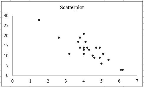
The relationship between two variables Temperature and first blossom days in April can be described on the basis of scatter plot.
Associated variables:
Two variables are associated or related if the value of one variable gives you information about the value of the other variable.
From the above obtained scatter plot, it is seen that the two variables Temperature and first blossom days in April are associated variables.
Direction of association:
If the increase in the values of one variable increases the values of another variable, then the direction is positive. If the increase in the values of one variable decreases the values of another variable, then the direction is negative.
Here, the values of days decrease with the increase in the values of temperature and the values of day’s increases with the decrease in the values of temperature.
Hence, the direction of the association is negative.
Form of the association between variable:
The form of the association describes whether the data points follow a linear pattern or some other complicated curves. For data if it appears that a line would do a reasonable job of summarizing the overall pattern in the data. Then, the association between two variables is linear.
From the scatter plot, it is observed that the pattern of the relationship between the variables Temperature and first blossom days in April is slightly linear.
Hence, there is a linear association between the variables Temperature and first blossom days in April.
Strength of the association:
The association is said to be strong if all the points are close to the straight line. It is said to be weak if all points are far away from the straight line and it is said to be moderate if the data points are moderately close to straight line.
From the scatter plot, it is observed that the variables will have perfect
Hence, the association between the variables is strong.
Hence, there is a strong, negative, linear association between the variables Temperature and first blossom days in April.
Conclusion:
There is a strong, negative, linear association between the variables Temperature and first blossom days in April.
(b)
To find: The equation of least square regression line.
(b)
Answer to Problem 5CRE
The intercept of the regression equation is 33.1203.
Explanation of Solution
Given information:
Use technology the equation of the least squares regression line is to be interpreted.
Formula used:
A simple linear regression model is given as y^ = b0 + bx + e
Calculation:
Regression equation to predict repair time given the repair type:
Simple linear regression model:
A simple linear regression model is given as y^ = b0 + bx + e
Where y^ is the predicted value of response variable, and x be the predictor variable. The quantity b is the estimated slope corresponding to x and b0 is the estimated intercept of the line, from the sample data.
Simple regression model can be build using EXCEL software:
Software Procedure:
The step-by-step procedure to obtain simple regression model using EXCEL software is given below:
- Open an EXCEL file.
- Enter the data values of Temperature (0C) in column A and name it as Temperature.
- Enter the data values of Days in column B and name it as Days.
- Click on Data > Data Analysis > Regression.
- In Input Y
Range enter $B$1:$B$25. - In Input X Range enter $A$1:$A$25.
- Click on
- Click OK.
The generated output is given below:
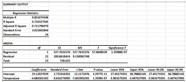
From the generate output, the intercept b0 = 33.1203 and slope coefficient b = -4.6855.
Thus, the simple linear regression equation to predict the first blossom days in April (y) given the temperature is Days = 33.1203 − 4.6855*Temperature.
Interpretation of slope:
The slope of the regression equation is -4.6855.
For any 1 unit increase in temperature, the number of days decreases by -4.6855 units.
Interpretation of intercept:
The intercept of the regression equation is 33.1203.
The number of days will be 33.1203 even when the temperature is 0.
Conclusion:
The intercept of the regression equation is 33.1203.
(c)
To analyse: The occurrence of the first cherry blossom.
(c)
Answer to Problem 5CRE
The predicted first cherry blossom day when the temperature is 3.50C is 17.
Explanation of Solution
Given information:
The average March temperate; this year was 3.5°C.
Formula used:
Calculation:
Predict the first cherry blossom day when the temperature is 3.50C:
The predicted first cherry blossom day when the temperature is 3.50C is obtained as 17 from the calculation given below:
Thus, the predicted first cherry blossom day when the temperature is 3.50C is 17.
Conclusion:
The predicted first cherry blossom day when the temperature is 3.50C is 17.
(d)
Tofind: The residual value for the year.
(d)
Answer to Problem 5CRE
The residual for the year when the average March temperature was 4. 50C is 2.
Explanation of Solution
Given information:
The average March temperate; this year was 4.5°C.
Formula used:
Calculation:
Predict the first cherry blossom day when the temperature is 4.50C:
The predicted first cherry blossom day when the temperature is obtained as given below:
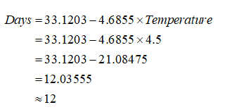
Thus, the predicted first cherry blossom day when the temperature is 4.50C is 12.
Residual for the year when the average March temperature was 4. 50C :
The residual for the year when the average March temperature was 4. 50C is obtained as 2 from the calculation given below:
Thus, the residual for the year when the average March temperature was 4. 50C is 2.
Conclusion:
The residual for the year when the average March temperature was 4. 50C is 2.
(e)
To construct: The residual plot.
(e)
Answer to Problem 5CRE
From the obtained residual plot it is observed that, the data points are deviating from the straight line.
Explanation of Solution
Given information:
The residual plot needs to be constructed.
Formula used:
EXCEL software
Calculation:
Residual plot can be build using EXCEL software:
Software Procedure:
The step-by-step procedure to obtain simple regression model using EXCEL software is given below:
- Open an EXCEL file.
- Enter the data values of Temperature (0C) in column A and name it as Temperature .
- Enter the data values of Days in column B and name it as Days .
- Click on Data > Data Analysis > Regression.
- In Input Y Range enter $B$1:$B$25.
- In Input X Range enter $A$1:$A$25.
- Click on
- Click on Residual plots.
- Click OK.
The generated output is given below:
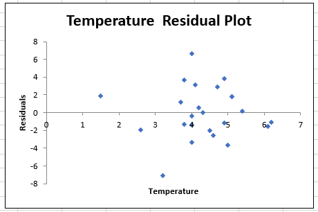
Observation: From the obtained residual plot it is observed that, the data points are deviating from the straight line. Therefore, the regression model does not seem of doing a very good job in predicting the days in April until the first blossom.
Conclusion:
From the obtained residual plot it is observed that, the data points are deviating from the straight line.
(f)
To find: The interpret value of r2
(f)
Answer to Problem 5CRE
The standard error in the regression model is 3.0216.
Explanation of Solution
Given information:
The values of r2 and s need to analyse.
Formula used:
The percentage of variation in the observed values of dependent variable
Calculation:
From the obtained regression output, the value of R-square is 0.7243.
R-squared:
The percentage of variation in the observed values of dependent variable that is explained by the regression is 72.43%, which indicates that 72.43% of the variability in the variable “First blossom days in April(Y)” is explained by the variability in independent variable “Temperature (X)” using the linear regression model.
From the obtained regression output, the value of standard error is 3.0216.
The standard error in the regression model is 3.0216.
Conclusion:
The standard error in the regression model is 3.0216.
Chapter 3 Solutions
The Practice of Statistics for AP - 4th Edition
Additional Math Textbook Solutions
Intro Stats, Books a la Carte Edition (5th Edition)
Introductory Statistics
Fundamentals of Statistics (5th Edition)
Introductory Statistics (2nd Edition)
Elementary Statistics
Statistics: The Art and Science of Learning from Data (4th Edition)


 MATLAB: An Introduction with ApplicationsStatisticsISBN:9781119256830Author:Amos GilatPublisher:John Wiley & Sons Inc
 Probability and Statistics for Engineering and th...StatisticsISBN:9781305251809Author:Jay L. DevorePublisher:Cengage Learning
 Statistics for The Behavioral Sciences (MindTap C...StatisticsISBN:9781305504912Author:Frederick J Gravetter, Larry B. WallnauPublisher:Cengage Learning
 Elementary Statistics: Picturing the World (7th E...StatisticsISBN:9780134683416Author:Ron Larson, Betsy FarberPublisher:PEARSON
 The Basic Practice of StatisticsStatisticsISBN:9781319042578Author:David S. Moore, William I. Notz, Michael A. FlignerPublisher:W. H. Freeman
 Introduction to the Practice of StatisticsStatisticsISBN:9781319013387Author:David S. Moore, George P. McCabe, Bruce A. CraigPublisher:W. H. Freeman