Concept explainers
Videos
To find: the accurate of DR.G’s forecasts and the number of tropical storms and the effect of the disastrous
Answer to Problem 69E
DR.G’s forecasts are not very accurate.
There are 16tropical storms
The effect of the disastrous has a little effect.
Explanation of Solution
Given:
| year | forecast | actual | year | forecast | actual |
| 1984 | 10 | 12 | 1997 | 11 | 7 |
| 1985 | 11 | 11 | 1998 | 10 | 14 |
| 1986 | 8 | 6 | 1999 | 14 | 12 |
| 1987 | 8 | 7 | 2000 | 12 | 14 |
| 1988 | 11 | 12 | 2001 | 12 | 15 |
| 1989 | 7 | 11 | 2002 | 11 | 12 |
| 1990 | 11 | 14 | 2003 | 14 | 16 |
| 1991 | 8 | 8 | 2004 | 14 | 14 |
| 1992 | 8 | 6 | 2005 | 15 | 27 |
| 1993 | 11 | 8 | 2006 | 17 | 9 |
| 1994 | 9 | 7 | 2007 | 17 | 14 |
| 1995 | 12 | 19 | 2008 | 15 | 16 |
| 1996 | 10 | 13 |
Calculation:
Let's start by making a
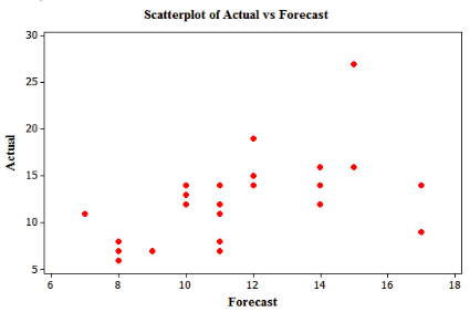
The below figure shows a scatterplot of the data. The scatterplot shows a positive association That is, higher number of forecast tends to have higher number of actual storms. The overall pattern is moderately linear (a calculator gives r = 0.5478). There is one outlier on the scatterplot in the Y direction.
Using the MINITAB, the regression equation is shown below
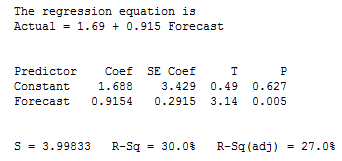
The least-square equation is
Using the MINITAB, the residual plot is shown below:
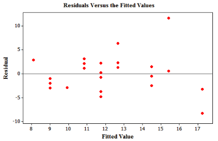
The slope suggests that for every added forecast, actual forecast increased by 0.915. Y intercept is the value of Y when X = 0, here if forecast is O then number of actual storm will be 1. From the residual plot. The graph shows a fairly "random" scatter points around the "residual = 0" line with one very large positive residual (point for year 2005). Most of the prediction errors (residuals) are 10 points or fewer on the forecast scale. It is calculated the standard error of the residuals to be s = 3.9983. This is roughly the size of an average prediction error using the regression line. Since
Use the equation
Actual storm = 1.69+0.915(forecast)
To predict an actual number of storm from the forecast. Our predictions may not be very accurate, though. It is hesitated to use this model to make predictions. If Dr. Gray's preseason forecast call is 16 then;
Actual storm
Consider the below figure:
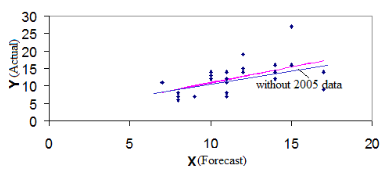
The above figure shows the result of removing 2005 season on the
Conclusion:
Therefore,
DR.G’s forecasts are not very accurate.
There are 16tropical storms
The effect of the disastrous has a little effect.
Chapter 3 Solutions
The Practice of Statistics for AP - 4th Edition
Additional Math Textbook Solutions
Introductory Statistics (2nd Edition)
Statistical Reasoning for Everyday Life (5th Edition)
Elementary Statistics: Picturing the World (6th Edition)
Elementary Statistics Using Excel (6th Edition)
Intro Stats, Books a la Carte Edition (5th Edition)


 MATLAB: An Introduction with ApplicationsStatisticsISBN:9781119256830Author:Amos GilatPublisher:John Wiley & Sons Inc
 Probability and Statistics for Engineering and th...StatisticsISBN:9781305251809Author:Jay L. DevorePublisher:Cengage Learning
 Statistics for The Behavioral Sciences (MindTap C...StatisticsISBN:9781305504912Author:Frederick J Gravetter, Larry B. WallnauPublisher:Cengage Learning
 Elementary Statistics: Picturing the World (7th E...StatisticsISBN:9780134683416Author:Ron Larson, Betsy FarberPublisher:PEARSON
 The Basic Practice of StatisticsStatisticsISBN:9781319042578Author:David S. Moore, William I. Notz, Michael A. FlignerPublisher:W. H. Freeman
 Introduction to the Practice of StatisticsStatisticsISBN:9781319013387Author:David S. Moore, George P. McCabe, Bruce A. CraigPublisher:W. H. Freeman